Trick/Tip: A Feedforward Neural Network with Neurons with "arbitrary" gradient/functions and connections

Decades ago I worked on experimental Pattern Recognition (Handwritten Character and Word Recognition) and I did also some small experiments with Neural Networks. I had some simple but well tested software ((in VMS Pascal :=) ) but code and datasets are gone by now.

 

In that time vanishing gradients, LSTM with error carousels and deep learning were not mainstream yet. Note that nowadays frameworks for deep learning are publicly available (hey, might even work on your graphic card)

 

When I read an article that applied deep learning I was curious how a Feedforward Neural Network with arbitrary Neuron Functions in C# would look like. For nostalgic reasons I decided as a little hobby project to make a first iteration /implementation /design in C# for the network and neurons. This trick/tip presents:

Later I was curious if an optimal step in the gradient was easy to implement so I added a sketchy implementation of a training Algorithm.

 

Since I had no practical application with experiments on real datasets in mind this was a very low priority and never ending project. I decided to end this project by publishing this code as a CodeProject trick/tip because the approach with "arbitrary" gradient/functions and the first design considerations might be of some interest.

 

The emphasis of this trick/tip is on the Neuron class with  "arbitrary" functions ComputeOutput and ComputeGradient and the design considerations of the network and neuron with a first sketchy proof of concept implementation. The software is not intended for practical use.

 

When using standard QuickProp provisional test results on the XOR problem look a factor worse than reported by Fahlman, so I am not totally convinced that the implementation is correct. Please report major errors, although it is not likely that I make an an article from this trick/tip.

I assume that the reader is familiar with Feedforward Networks and its training. See for some popular C# stuff for example visualstudiomagazine. A Network of Neurons is used. A standard sigmoid Neuron computes a weighted sum of its inputs and then applies a sigmoid function to compute its output. Neurons are successively computed in a feedforward way using the network input and outputs of previous computed neurons.

Several topologies are possible for example

The weights/parameters of a network have to be trained. In Pattern Recognition we have often a Learning Set and a Test Set. On the Learning Set we train the parameters (fitting), ideally we use the Test Set once/sparsely to determine the score of the trained network (generalization).

 

Larger networks with lots of free weights/parameters will fit a learning set easier but can have worse generalisation on a test set with samples never seen before. This is similar with function approximation given n points. A nth order polynomial can fit the n points exactly, but the interpolation/generalisation on points outside the training data can be worse then for example a linear approximation.

 

Many classifiers exist in Pattern Recognition such as k-Nearest Neighbour, Tree, SVM, Forest Trees, AdaBoost etc. In the universe of problems there is no free lunch e.g. there is no universal best solution. On the other hand the universe of problems is in certain domains not random :=). So a neural network that is a universal function estimator has its use, and a neural network that approximates a known distribution at hand has also its use.  

 

It is interesting to note a linear plane (= a one layer network) in N dimensions is able to assign any N+1 samples with different input values any desired label (0/1), see also the VC dimension.  So in 2 dimensional space a one layer network can assign any 3 samples any desired label, but not any 4 samples (XOR problem). In higher dimensional feature spaces our intuition is not always correct and the linear plane can be adequate (see also the principle of SVM, enlarge the dimension of the feature space). If we use a one layer network to recognize a phoneme with for example its context using 15*16 = 240 inputs, it can assign any 241 different samples any label. Normally data of the same class is clustered, so if there is enough separation in feature space we could theoretically cover 241 clusters.

 

However sometimes a higher VC dimension is needed. Sometimes it can also be useful to incorporate some knowledge into the network. In some domains representation ( features) is crucial and it can be beneficial to train  in a competitive way for example the moving filter "features" of a TDDN.

Suppose we choose a quadratic error measured over all Learning Samples L and the outputs of the C output neurons, see Figure 1. The desired value d for sample with a feature vector of x (network input) is 1 if the neuron depicts the desired class, otherwise 0.

 

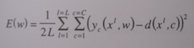
Figure 1. Error Criterion.

 
The derivative of E with respect to Yj of the output neurons of one sample can be computed, see figure 2 lower right formula. Next the neurons are handled in a backward direction compared to the Feedforward computation. Given the derivative of the Error with respect to a neuron output, the contribution to the derivative of E with respect to its inputs s can be computed by using the chain rule, see figure 2 top right formula.
 

Figure 2. Chain rule to backpropagate error from output neuron y to neuron input s (output neurons bottom-right formula, hidden neurons top-right formula)

 

It is possible to choose several functions y=F(w,s). By applying the chain rule it is possible to compute the derivative of E in respect to the weights. See figure 3 for some examples. Note that it is of course more efficient to use larger units then to construct a network with elementary multiplication, sum etc. neurons.

 

Figure 3. Some sample neurons and their derratives for inputs and weights.

 

The weighted distance is mentioned for a small experiment to find multiple clusters in the Timit database (failed, an optimised distance method behaves somewhat as a one layer Feedforward network), the max function is mentioned (not quite correct in the table, output derivative zero for non maximum inputs) because in one experiment I did optimize the selected substitution costs from the best path of a Minimal Edit Distance (so not really a max/min in the feedforward network).

 

• In the network an array y is used to store network input, output of the hidden neurons and output of the output neurons. As I remember this is convenient for implementing RNN.
• A minor decision is to implement in the neuron an integer yIndexOut, y[yIndexOut] depicts the value in the y array of the Neuron output. The neuron has only one output.
• In the network Weights (array wf) and derivatives (array dEdy and dEdwf) are stored. This is most convenient for the gradient search. With growing networks,  normalisation per neuron or for feedforward computing speed storing these weights (or a shadow copy) in the neurons could be more convenient.
• A minor decision is to implement in the neuron wL and wH, in wf[wL..wH] the weights/parameters of the neuron are stored.
• Connections from or to y can be coded in explicit as "for" loops in forward and backward direction. We have chosen to use per Neuron an yIndexIn[] array that is constructed in network initialisation. This will cost an extra array access in comparison to explicit for loops.
• In the neuron the array yIndexIn[] and integer yIndexInH are stored, yIndexIn[0..yIndexInH] are the indices of the inputs of the neuron in the y array. 

Networks and Neurons

    public interface INeuron
    {
        // wf, parameters for this Neuron in wf[wL..wH], wf[] in network
        int wL { get; set; }
        int wH { get; set; }

        IEnumerable<int> wfIndexNeuron();

        // connections from y[] of network to inputs of this neuron locally;
        // yIndexIn[0]..yIndexIn[xx]..yIndexIn[yIndexInH].
        int yIndexInH { get; set; }
        int[] yIndexIn { get; set; }

        IEnumerable<int> yIndexInAll();

        // Only one output per neuron.
        // Neuron outputs to y[yIndexOut] FeedForwardNetwork. Gradient dEdy in dEdy[yOutIndex].
        int yIndexOut { get; set; }

        // ComputeOutput uses wf[] and y[] of network to perform forward computation.
        // ComputOutput uses y[ yIndexIn[..] ] as neuron inputs, writes neuron output to y[yIndexOut] 
        // ComputeOutput abstract method, must be implemented in non abstract class, see neurons.cs 

        void ComputeOutput(double[] wf, ref double[] y);

        // given dEdy[yIndexOut] chain rule used to compute dEdy inputs(yIndexIn[]) 
        // and dEdwf of neurons parameters (wfIndexNeuron[])
        void ComputeGradientBackward(double[] wf, double[] y, ref double[] dEdy, ref double[] dEdwf);
    }

public interface IFeedForwardNetwork
{
    // Refinement: split interface for forward computation and backward gradient computation

    // y[0..yH] vector
    // y[] input sample + hidden + output map to y;

    // y[] used as input for Neurons, Neurons write to y[Neuron.yIndexOut]
    // y[] not in interface, no property since we can't use properties as procedure parameters;
    // in implementation public double[] y etc

    // double[] y { get; set; }
    // double[] dEdy { get; set; }

    int yH { get; set; }

    // y[0..xH] copy of input; y[hl..hH] output of Hidden Neurons; y[oL..yH] output Output Neurons
    int xH { get; set; }
    int hL { get; }
    int hH { get; set; }
    int oL { get; }
    int oH { get; }

    void SetNetworkDimensions(int nInput, int nHidden, int nOut);

    // Some Enumerable s to access ranges, use: foreach (int iInput in yIndexInputX()) {}
    IEnumerable<int> yIndexAll();
    IEnumerable<int> yIndexAllNotInputNeurons();
    IEnumerable<int> yIndexHiddenNeurons();
    IEnumerable<int> yIndexInputX();
    IEnumerable<int> yIndexOutputNeurons();

    // Some variables defined in Network class, but not as properties, so not in interface:
    // List<INeuron> Neurons;

    // wf[] all wf/parameters of network. Neurons access their own wf[]
    int wH { get; set; }
    // double[] wf { get; set; }
    // double[] dEdwf { get; set; }

    void ComputeNetworkFeedForward(ISample sample);

    // quadratic error outputs and desired outputs
    double ComputeError(int desiredLabel);

    // FeedForwardNetwork[0..], returns values output neurons
    double this[int index] { get; }

    // BestClass for Classification, Delta for reliable reject, dep. error criterion
    int BestClass();
    double DeltaOutput();

    // Computing Gradient, not in separate interface/child class:

    void InitRandomWf(double delta = 0.1);
    void ZerodEdw();

    // set dEdy output layer given criterion, init rest
    void SetdEdyFromDesiredOutput(int desiredLabel);

    // and compute dEdy and dEdWf by backwards propagation
    void ComputeNetworkGradientBackward(int desiredLabel, bool InitDeDw = false);

    // Normalize the gradient on the nrSamples, Gradients computed are summed
    void dEdwfNormalise(int nrSamples);
}

foreach (Neuron n in Neurons) n.ComputeOutput(wf, ref y);

for (int n = Neurons.Count - 1; n >= 0; n--)
     Neurons[n].ComputeGradientBackward(wf,y,ref dEdy, ref dEdwf);

• OneLayerNetwork(NrInputs, NrOutputs)
• CascadeNetwork(NrInputs,NrHidden,NrOutputs)
• FullyConnectedOneHiddenLayerNetwork
        (NrInputs,NrHidden,NrOutputs, Func<INeuron> CreateHidden, Func<INeuron> CreateOutput)CreateHidden, CreateOutput can be specified in function call by lambda expression: (.., ()=> new HalfTanhNeuron(), ()=> new SigmoidNeuron()). 

Tip: measuring run-times

Points of Interest

• We presented a first trial design of a feedforward network with neurons with "arbitrary" output/gradient and "arbritrary" feedforward connections.
• We discussed shortly some design decisions where to implement (in network, in neuron ) network input, output, output of hidden neurons , weights, connections etc.
• This first iteration trial can be used as a reference for a next iteration of the software.
• The software is not intended for practical use. There are deep learning frameworks already available.
• Before actually using the software similar results as reported by Fahlman should be obtained, which is a project of its own.
• Runtimes are not considered in this first try. Using a GNU package runtimes could be measured.
• It could be considered to pass the parent network as a function parameter or as property in the neuron. In this way each neuron can access weights etc. from the network directly.  
• The sample class that allows different kind of extra info is too complex, next iteration samples should be just a label and a feature vector.
• The approach does have some overhead in Neurons and calls to functions computeOutput() and ComputeGradient(). When using layers and in each layer standard neurons  a few explicitly coded for loops are more efficient in code size, complexity and runtimes .
• Separating the construction of the connections and the ComputeOutput() and ComputeGradient() makes it somewhat simpler to adapt the network and its neurons.

Appendix A. Samples and Basic IO

public interface ISample
{
    int xH { get;}
    // Pattern with feature vector x of float[]
    float[] x { get; set; }
}

public interface ISampleInfo
{
    int label { get; set; }
}

public interface ISampleWithInfo<TSampleInfo> : ISample where TSampleInfo : ISampleInfo
{
    TSampleInfo sampleInfo { get; set; }
}

public interface ISampleSet<out T>
{
    void First();

    T GetNextSample();
    bool IsLastSample();
}

Samples are normally just arrays of feature vectors and a label. As I remembered for many projects is was convenient to store extra project info the sample (logical info such as field, layout info such as sequence of rotated snippets to extract pattern from total image). For that reason I added the possibility to add some extra info to the sample using generetics. I did not consider Inversion of Control because I.M.O. generetics is a little more basic.

 

In samples.cs we define as an example two classes of samples, one using class MySampleInfo that contains only the required label, the other using MySampleInfo1 containing an additional id. In SampleSets an example of the definition of a Xor sample set we used for testing, for more details download code. Make sure that the SampleInfo of the sets used match the SampleInfo of the training class creation.  

public class XOrSampleSet1 : ListSampleSet<MySampleWithInfo1>
{
  override public void MakeList()
  {
    var x00 = new MySampleWithInfo1 { sampleInfo = new MySampleInfo1 { label = 0, id = 0 },
                                      x = new float[2] { 0, 0 } };
    var x01 = new MySampleWithInfo1 { sampleInfo = new MySampleInfo1 { label = 1, id = 2 },
                                      x = new float[2] { 0, 1 } };
    var x10 = new MySampleWithInfo1 { sampleInfo = new MySampleInfo1 { label = 1, id = 1 },
                                      x = new float[2] { 1, 0 } };
    var x11 = new MySampleWithInfo1 { sampleInfo = new MySampleInfo1 { label = 0, id = 3 },
                                      x = new float[2] { 1, 1 } };

     samples.Add(x00); NrSamples++;
     samples.Add(x01); NrSamples++;
     samples.Add(x10); NrSamples++;
     samples.Add(x11); NrSamples++;

     First();
  }
}

 

In the design of samples the emphasis was more on software exploration than simplicity. However the chosen approach is too complex and confusing and for educational reasons and to avoid errors,  the sample class could be simplified to a label and a feature vectorin the next iteration of the software.

public interface INetworkTraining<TSampleInfo> where TSampleInfo : ISampleInfo
{

  // - Training1() as sample uses default InitTraining1() which sets parameters
  // - Alternatively all parameters can be set and then use: InitTraining1=false; Training1(useInitTraining1)
  // - Training1() can also be overwritten in child class

  int nrMaxIterations { get; set; }
  int nrTrainingSamples { get; set; }

  ISampleSet<ISampleWithInfo<TSampleInfo>> learningSet { get; set; }
  ISampleSet<ISampleWithInfo<TSampleInfo>> testSet { get; set; }
  ISampleSet<ISampleWithInfo<TSampleInfo>> stopSet { get; set; }

  FeedForwardNetwork ffNet { get; set; }

  Training.QuickProp quickProp { get; set; }

  void ComputeGradient(ISampleSet<ISampleWithInfo<TSampleInfo>> learningSet, FeedForwardNetwork ffNet);

  int ComputeScoreSet(ISampleSet<ISampleWithInfo<TSampleInfo>> testSet, FeedForwardNetwork ffNet);

  double ComputeErrorOnSet(ISampleSet<ISampleWithInfo<TSampleInfo>> _Set, FeedForwardNetwork _ffNet);

  void AdaptWeightsUsingGradient();
  void AdaptWeightsGradientWithOptimalStepSize();

  //
  // Methods called (or overridden in child class) for training

  // refinement: stopTrainingAsap can be external set to stop training
  // does not work yet, UI blocks?, start training on other thread?
  bool stopTrainingAsap { get; set; }

  // virtual methods, can be overwritten in child class
  bool ContinueTraining(int iIter);
  bool ContinueTrainingWithStopSet(int iIter, int errorStopSet, int MaxIterationsNoImprovement = 100);

  void ReportEveryIteration();
  void ReportFinalResults();

  // For running sample use Training1()
  // Other possibility specify parameters first and then call Training1(false)
  // Otherwise define derived child class and redefine Training 1 etc.
  // ... or define your own network training module ;=)

   void InitTraining1();
   void Training1(bool useInitTraining1 = true);
}

public interface IQuickProp
{
    // Set nrWf, required!!
    int nrWf { get; set; }

    // Internal used variables in Step algorithm
    double[] dEdwOld { get; set; }
    double[] deltawOld { get; set; }

    double stepOld { get; set; }

     ...

    // Magic but crucial Quickprop training parameters
    // Note that the initial settings of weights (random size) is also crucial parameter
    double epsilon { get; set; }
    double mu { get; set; }
    double decay { get; set; }

    // double[] generalParameterSettings = new double[3] { 0.1, 1.0, 0.0001 };
    // //public double[] xorParameterSettings = new double[3] { 4.0, 2.25, 0.0001 };
    // //No epsilon sharing; normalisation to nr samples in Fahlman??:
    //double[] xorParameterSettings = new double[3] { 1.0, 2.25, 0.0 };


    double[] GetCurrentParameters();
    void SetCurrentParameters(double[] parameters);

    // GradientStep
    void WfAdaptFirstStep(ref double[] wf, double[] dEdwf, double gradStart = 0.1);
    void WfAdaptQuickPropStep(ref double[] wf, double[] dEdwf);
}

 

UtilDeepCloneCopy.cs and UtilGoldenSectionSearch1D.cs where added for a proof of concept of how to incorporate an optimal gradient step. However the GoldenSectionSearch is probable not a correct implementation, I did not take time to understand the algorithm properly. Better is to use the Brent search algorithm.

 

• EntropieOutputNeuron. Sigmoid, linear derivative.
• FlatSpotOutputNeuron. Sigmoid, 0.1 + standard sigmoid derivative as described in Fahlman's report. At first sight that can be considered as a weighted sum of M.S.E. and entropy criterion.
• ArcTanhOutputNeuron. FlatspotNeuron, but non linear processing of the error by taking dedy=ArcTanh(dedy) as I understand from Fahlman's report. The ArcTanh on the derivative seems at first sight behave somewhat as the EntropieOutputNeuron, but combination of 0.1 + standard sigmoid derivative I do not understand that yet, although it might work.