
Understanding Logistic Regression with ML.NET
5.00/5 (7 votes)
How to implement logistic regression in ML.NET?
Introduction
In machine learning, classification tasks refer to the process of categorizing input data into predefined classes or categories based on their features. The goal is to train a model that can learn patterns and relationships in the data, allowing it to make predictions or assign labels to new, unseen instances.
Classification tasks are prevalent in various domains, such as spam detection (classifying emails as spam or not spam), image recognition (identifying objects or patterns in images (e.g., recognizing digits in handwritten digits recognition) or sentiment analysis (determining the sentiment (positive, negative, neutral) in textual data).
Among the various algorithms employed for classification tasks, commonly used ones include decision trees, support vector machines, k-nearest neighbors, and neural networks. In this series, we will delve into classical logistic regression, highlighting the inherent mathematical intricacies associated with this technique.
This article was originally posted here. Refer to this site for a more comfortable reading.
What is Supervised Learning?
Supervised learning is a type of machine learning paradigm where the algorithm is trained on a labeled dataset, which means the input data used for training is paired with corresponding output labels. The goal of supervised learning is for the algorithm to learn the mapping or relationship between the input features and the corresponding output labels. Once the model is trained, it can make predictions or decisions when given new, unseen input data.
The process involves the following key steps:
-
A labeled dataset is used for training, consisting of input-output pairs. The input represents the features or attributes of the data, while the output is the labeled or desired outcome.
-
An algorithm processes the training data to learn the patterns and relationships between the input features and output labels. During this training phase, the algorithm adjusts its internal parameters to minimize the difference between its predictions and the actual labels.
-
Once trained and validated, the model can be used to make predictions or decisions on new, unseen data. It takes the input features and generates output predictions based on the learned patterns.
Supervised learning is itself categorized into two main types: regression and classification.
Example of Regression
In a regression task, the algorithm predicts a continuous value or quantity. As an example, we can forecast the price of a house by considering its size (in square meters). A sample of training data is presented below.
| Size (in square meters) | Price (in $) |
| 120 | 500000 |
| 40 | 100000 |
| 42 | 105000 |
| 64 | 165000 |
| 76 | 185000 |
| 55 | 145000 |
| ... | ... |

This example exemplifies precisely what we've defined: the training data is merely the table above with one input variable (size) and one output variable (price). The next step involves selecting an algorithm to establish the relationship between this input and output, enabling us to predict unforeseen data. For instance, we could determine the price of a 100-square-meter house using this trained model.
Example of Classification
In a classification task, the algorithm assigns input data to predefined categories or classes. As an illustration, we can predict the gender (M or W) of an individual by taking into account their height (in centimeters). A sample of training data is presented below.

This data highlights the challenge of a classification task. It is evident from the chart above that predicting the gender of an individual who is 172 centimeters tall is not straightforward—it could be either a man or a woman. Instead, the idea is to determine a probability for an individual to be a man or a woman based on their height. In mathematical terms, we aim to predict P(M∣h), and given the binary nature of the classes, we can also express that P(W∣h)=1−P(M∣h).
Disclaimer 1
The latter situation is unrealistic. In a real-world context, there would typically be multiple observed variables, such as weight or foot size, for instance. However, calculations become more intricate in multidimensions, visualizations are more challenging to depict, and for illustrative purposes, we intentionally confine ourselves to a one-dimensional perspective.
Disclaimer 2
The example we used here pertains to a binary classification between two classes. However, it's important to note that the principles we're outlining remain applicable for scenarios involving K classes, where K>2.
In the subsequent parts of this series, our emphasis is directed toward classification tasks.
Enter the Bayes' Theorem
Bayes' theorem is a fundamental principle in probability theory that describes the probability of an event based on prior knowledge of conditions that might be related to the event. Named after the Reverend Thomas Bayes, who formulated the theorem, it is particularly useful in updating probabilities when new evidence becomes available.
The theorem is expressed mathematically as P(A∣B)=P(B∣A)P(A)/P(B)
- P(A∣B) is the probability of event A occurring given that event B has occurred.
- P(B∣A) is the probability of event B occurring given that event A has occurred.
- P(A) is the prior probability of event A.
- P(B) is the prior probability of event B.
Bayes' theorem allows us to update our belief in the probability of an event (A) based on new evidence (B).
Applying Bayes's theorem to our earlier classification task, we can express it as P(M∣h)=P(h∣M)P(M)/P(h)).
From this point, we can utilize the law of total probability to represent P(h). Indeed, men and women form are a set of pairwise disjoint events whose union is the entire sample space.
P(h)=P(h∣M)P(M)+P(h∣W)P(W)

We are simply engaging in a straightforward rewriting of mathematical functions, and at first glance, this process may appear somewhat trivial. However, firstly, it serves the purpose of demonstrating that the sigmoid function is not arbitrarily chosen but emerges naturally in the formulas. Moreover, we will explore specific cases to illustrate the judiciousness of such rewrites.
What Happens if the Distribution Is Gaussian?
In the preceding formulas, we need to specify the values of P(h∣M, P(h∣W), P(M) and P(W).
- The P(h∣M) and P(h∣W) quantities represent class-conditional probabilities: given that we are in the M category for example, what is the distribution of probabilities ?
A picture is worth a thousand words, so let's visualize the distribution of points belonging to the M category.

The distribution bears a strong resemblance to a Gaussian, indicating that we can effectively model the class-conditional probability using such a distribution.
Similarly, we can model the class-conditional probability for the W category.

Once again, the distribution bears a strong resemblance to a Gaussian, indicating that we can effectively model the class-conditional probability using such a distribution.
Therefore, by incorporating all these formulas into the calculations above, we can ultimately express P(M∣h) leading to a linear function of h in the argument of the sigmoid.
P(M∣h)=σ(wh+b)
What Happens With Discrete Features?
In the case of the Bernoulli distribution, for example, we can demonstrate that the outcome is still a linear function of the features in the argument of the sigmoid. Readers interested in a detailed proof of this assertion can refer to Pattern Recognition and Machine Learning.
Under rather general assumptions, the posterior probability of class C1 can be written as a logistic sigmoid acting on a linear function of the feature vector ϕ so that P(C1∣ϕ)=σ(wTϕ).
Christopher Bishop (Pattern Recognition and Machine Learning)
What Is Logistic Regression?
The goal is to extend the previous findings by stipulating that the outcome P(C∣inputvariables) is a linear function of the features within the sigmoid's argument. It's important to note that we do not assume the class-conditional probabilities to follow a Gaussian or Bernoulli distribution. Instead, we draw inspiration from these models to prescribe the probability.
This method of a priori imposing a linear function of features for the sigmoid is termed logistic regression. The sigmoid is sometimes termed as the link function.
Important 1
This approach can be more broadly generalized by allowing flexibility in choosing the link function (in this case, we mandated it to be a sigmoid). This extension gives rise to the concept of a generalized linear model (GLM), a topic extensively explored in the literature.
Important 2
Logistic regression belongs to the family of models known as discriminative models. In this approach, we a priori impose the probability of the outcome without making specific assumptions about the class-conditional probabilities, and we do not employ Bayes' theorem. In contrast, models that start by modeling class-conditional probabilities are referred to as generative models.
Now, let's explore how to calculate the introduced parameters (W and b). To illustrate these concepts, we will assume binary classification with classes C1 and C2, with the training dataset D comprising N records (x1, ..., xN), each encompassing K features (observed variables).
Introducing the Cost Function

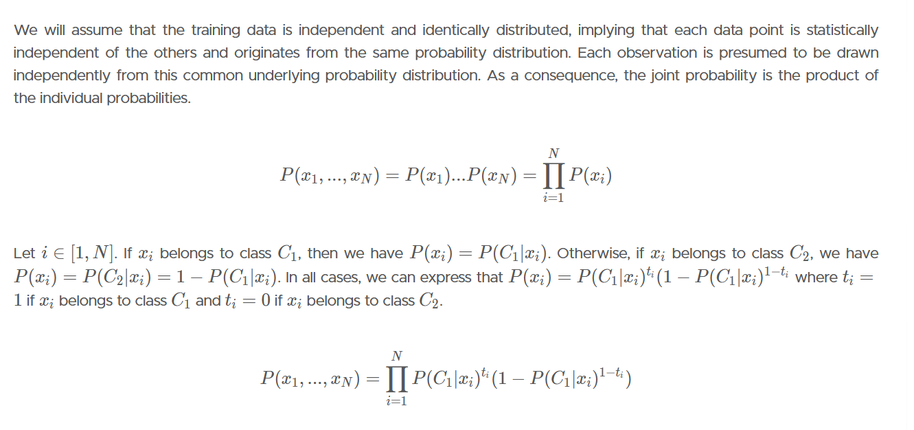
Information
This quantity is referred to as the likelihood.
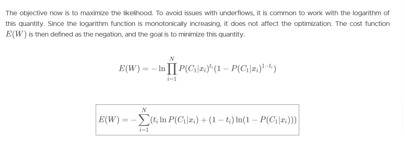
Minimizing the Cost Function
What we aim to do now is minimize the cost function. There are various methods for achieving this, such as different variants of gradient descent. In this post, we will choose to leverage the Newton-Raphson method by observing that minimizing E involves nullifying its gradient.
∇E(w)=0
In this approach, we turn to the task of identifying the roots of a non-linear equation, and it is in this context that the Newton-Raphson method becomes instrumental.
Very Important
Several optimization algorithms are possible, and the most commonly used ones are probably variants of gradient descent (such as stochastic gradient descent, conjugate gradient). Here, we present a method that leverages the Newton-Raphson algorithm.
What is the Newton-Raphson Method ?
The mathematical details of the Newton-Raphson method are elaborated in the original paper. Simply note that the convergence is very rapid, enabling the parameters to be learned quickly through these iterations.
Information 1
This algorithm is sometimes referred to as the iterative reweighted least squares (IRLS).
Information 2
We have presented the framework for binary classes here. All these findings can be extended to KK classes, where the link function is no longer a sigmoid but the softmax function. The Newton-Raphson method can still be utilized to train the parameters in this generalized context.
How to Predict an Unforeseen Input?
Once the logistic regression has been trained using the Newton-Raphson method, it becomes possible to make predictions. From an input xx, we can calculate the probability for each class Ck using the formula derived earlier (P(Ck∣x)=σ(WTx) and select the category with the highest probability as the predicted outcome.
Certainly, enough theory for now. It's time to put this knowledge into practice. Let's apply these formulas using the ML.NET framework. To avoid overloading this article, readers interested in this implementation can find it here.
History
- 4th January, 2024: Initial version