Real-Time Data Science and BI with Azure Synapse Analytics Part 3: Performing Real-Time Data Science and Business Intelligence

In the first article of this series, we discussed ways to analyze real-time data without affecting application performance. In the second article, we prepared our Azure Cosmos DB account, added sample retail sales data, created an Azure Synapse workspace, and linked Azure Synapse Studio.

Here, we will set up Power BI to display our data, helping us gain insight into our retail sales performance.

Querying the Data

Let’s start by querying our retail sales data using Synapse Apache Spark. Gestures in the Azure Synapse Studio provide sample code to quickly start querying data from the linked Azure Cosmos DB database. We can access gestures through the Actions context menu in the Data tab. The images below show the motions of the SalesData and SalesDataHTAP containers we created in the previous article:

We see that in the most general case (HTAP-enabled container), we can query data in three ways:

• Load to DataFrame: In this case, Synapse Analytics imports the data as the dataframe. It caches data through the Spark session’s lifetime. This means Azure Synapse takes the analytical store snapshot to the dataframe. For this reason, Azure Synapse evaluates all operations we perform on the dataframe against this snapshot. Practically, when we update data in the analytical store, we will not see an update in the dataframe.
• Create Spark table: Contrary to the previous case, Azure Synapse imports data from the analytical store into a Spark table. The data reloads from the underlying store on every execution of the query we perform against the Spark table.
• Load streaming DataFrame from the container: Azure Synapse loads the data from the analytical store into a dataframe and stores it in the primary data lake account — the one we configured when creating the Azure Synapse workspace.

Creating a Spark Table and Analyzing Data

To demonstrate importing the data, let’s create the Spark table from the SalesDataHTAP. To do so, we use the Create Spark table gesture, which generates the following code:

%%sql
-- Create a Spark table over Cosmos DB analytical store
-- To select a preferred list of regions in a multi-region Cosmos DB account, add spark.cosmos.preferredRegions '<Region1>,<Region2>' in the config options
 
create table YOURTABLE using cosmos.olap options (
    spark.synapse.linkedService 'CosmosDb_Sales_Info',
    spark.cosmos.container 'SalesDataHTAP'
)

We modify this gesture by replacing the YOURTABLE placeholder with SalesDataHTAP:

Before we can run the notebook, we need to attach the Apache Spark pool. We can do this through the Manage tab of Synapse Studio. However, we can quickly go to this view using the Manage pools option from the Attach to dropdown list (see the upper part of the above screenshot). This option takes us to another view, where we either click the Create Apache Spark pool button or the + icon.

The Apache Spark pool configuration pane appears on the right. We use this pane to configure the new pool.

We use the following values:

• Apache Spark pool name: synapseap
• Node size: small
• Autoscale: disabled
• Number of nodes: three

After setting up the Apache Spark pool, we can create the new synapseap pool (Apache Spark pool name) and launch the notebook by clicking the Run all button:

It takes a short while to get data from the Azure Cosmos DB. We should see output similar to the following:

We will now use the imported data. Let’s create a new cell (click the + icon below the output, and choose Code cell). Then, let’s add the following code to import the data to the dataframe and display all columns:

df = spark.sql("SELECT * FROM SalesDataHTAP")
display(df)

After we execute this code, we should see the following output:

Of course, we can use the dataframe to perform further analysis. For instance, we can count the items per year:

df.groupBy('Year').count().show()

It produces output like below:

The resulting table shows the number of items per year. They sum up to 10 because we have 10 items in our Azure Cosmos DB.

Note that the above approach will not work for the SalesData container because it does not support live snapshots. If we try to run the above code against this container, we will see the following error:

In summary, when we create the Spark table, it appears on the Data tab, under the Workspace/Database group. From there, we can access more gestures that enable us to start quickly. For instance, we can use the New notebook/Load to DataFrame gesture to generate the code for loading data from a table to a dataframe (like the one we used above), or use machine learning gestures:

We can also drop the table anytime using the following statement:

spark.sql("SELECT * FROM <TABLE_NAME>")

Loading a Snapshot to DataFrame

After learning how to use the Spark table, we will see how to take the snapshot of the analytical store into a dataframe. To do so, we can use the Load to DataFrame gesture. It generates the following code:

# Read from Cosmos DB analytical store into a Spark DataFrame and display 10 rows from the DataFrame
# To select a preferred list of regions in a multi-region Cosmos DB account, add .option("spark.cosmos.preferredRegions", "<Region1>,<Region2>")
 
df = spark.read\
    .format("cosmos.olap")\
    .option("spark.synapse.linkedService", "CosmosDb_Sales_Info")\
    .option("spark.cosmos.container", "SalesDataHTAP")\
    .load()
 
display(df.limit(10))

Let us modify this default code to add the aggregation we had in the previous section (df.groupBy('Year').count().show()). Of course, the output looks the same:

However, the difference between the two approaches will reveal itself when we update the underlying analytical store.

Updating the Analytical Store

So far, we successfully fetched the data using two different approaches and performed a simple aggregation. Let’s now see the actual difference to demonstrate the advantages of Azure Synapse Link for Azure Cosmos DB.

To this end, we will now modify the data we have in Azure Cosmos DB. The easiest way to do so is to use our ImportSalesData notebook and insert more than 10 items into a table. We can change the data_count from 10 to 30 and re-run the notebook under the Azure Cosmos DB:

Let’s now go back to Azure Synapse Studio and run the notebook that uses the Load to DataFrame gesture. We will see that the output does not change, even after refreshing the entire CosmosDb_Sales_Info link. The snapshot of the data we captured a few moments ago will be active for the whole Spark session. The only way to refresh the information is to start a new session.

However, if we now go back to the first notebook that uses a Spark table, we can refresh the data without restarting the Spark session:

Refreshing the data, though, might sometimes require recreating the table. Remember, you can drop the existing table with the following statement:

spark.sql("DROP TABLE SalesDataHTAP")

Previewing Data

In the above example, we used a relatively simple method to aggregate and present our sales data in a simple table. With Azure Synapse Studio, we can quickly do much more, like making customizable charts without code. Making these charts works quite similarly to Azure Machine Learning Studio. So, if you are familiar with that tool, you can easily switch to Azure Synapse Studio.

To demonstrate this capability, we load the data from the table to the dataframe, then display it:

df = spark.sql("SELECT * FROM default.salesdatahtap")
 
display(df)

The resulting data displays in the table. We use the View switch to change the default setting from Table to Chart. Then, we open View options (a small icon in the top right corner). It opens another pane, where we configure the options as follows:

• Chart type: column chart
• Key: country
• Values: price
• Series Group: year
• Aggregation: sum
• Stacked: checked
• Aggregating overall results: unchecked

The figure below shows this configuration, along with the sample result:

Our chart displays annual sale prices by country.

Creating Charts in Power BI

If we need more comprehensive data visualization, we can further link Azure Synapse Studio with Microsoft Power BI. We can then build interactive Power BI charts from our data the same way as Power BI Desktop or the Power BI service. Specifically, we use Azure Synapse Studio to generate the downloadable dataset.

To create this dataset, we use a dedicated SQL Pool within Azure Synapse Studio. Once we have this pool, we import the required data. We can first perform data cleaning or aggregation in practice, then create a new table in a dedicated SQL Pool.

Based on that, Azure Synapse Studio creates a *.pisb file, which we download and then import into Power BI Desktop. We then use this data to produce our report, which will become available in Azure Synapse Studio after publishing to the workspace. This path requires us to install the Power BI Desktop, so we need a machine with Windows 10.

We can find all installation requirements and details in Microsoft documentation.

First, we need to link Power BI with Azure Synapse Studio. We go to the Manage tab and click Linked services on the left, from where we click + New:

We see that a yellow rectangle with a Connect to Power BI button links with Power BI. After we click this button, we need to provide the service name and subscription. Here, we set the service name to PowerBiSynapseDemo, and under Power BI, create a workspace named SynapseDemo.

Note that to make this work, you need a Power BI Pro license to create workspaces in the Power BI service. We will need to have a Pro license, or else sign up for a one-month free Power BI Pro trial.

The image below summarizes our configuration where we used SynapseDemo Power BI workspace:

Once we finish configuring Power BI, we click Save, then the Publish all button in Manage/Linked services.

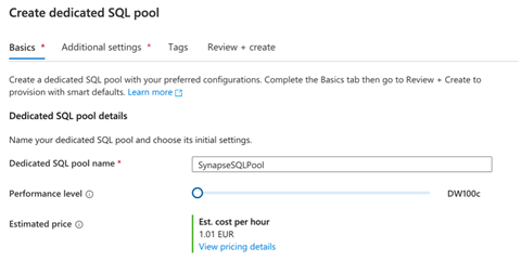
Now, we need to create a dedicated SQL pool. To do so, we follow the instructions in Microsoft documentation. We go to the Manage tab then click SQL Pools/New. Afterward, we name our pool (for example, SynapseSQLPool) and choose our performance level. Here, we set performance to DW100c to minimize the cost:

To proceed further, we need to copy data to this dedicated SQL pool. Then, we generate the dataset, which we can import into Power BI Desktop.

Azure Synapse Studio provides a connector enabling data transfer from a dataframe to a table in the dedicated SQL pool. Currently, this connector is only available for Scala.

To compensate for this, we first load data from Azure Cosmos DB into a dataframe. Afterward, we filter this dataframe and save the results to a Spark table. We use another Scala notebook cell to read the table from Spark then save it to SynapseSQLPool.

Here is the code for the first step:

# Load data from Cosmos DB to Spark table
df = spark.read\
    .format("cosmos.olap")\
    .option("spark.synapse.linkedService", "CosmosDb_Sales_Info")\
    .option("spark.cosmos.container", "SalesDataHTAP")\
    .load()
 
# Select interesting columns and filter out '0' Year
df_filtered = df.select("Year","Price","Country").where("Year > 0")
 
# Display data
display(df_filtered)
 
# Write data to a Spark table
df_filtered.write.mode("overwrite").saveAsTable("default.sales")

This code produces an output similar to what the following figure shows:

We should also see the sales table in the Data tab (workspace/default (Spark)/Tables/sales).

Now, we create another cell, which copies the data from the Spark table to a dedicated SQL pool:

%%spark
val scala_df = spark.sqlContext.sql("select * from sales")
 
scala_df.write.synapsesql("synapsesqlpool.dbo.sales", Constants.INTERNAL)

After running the cell, we should see the new table in the SQL pool:

We can go ahead and confirm the data is there. We just use the New SQL script/SELECT TOP 100 rows gesture from the Actions context menu of dbo.sales. It creates the SQL query. After this query executes, it produces the output in the image below:

Now, when the data is in our SQL pool, we can create the Power BI report. We need to go to the Develop tab. It now contains the Power BI group, under which we can find our workspace (for example, PowerBIWorkspaceSynapseDemo). The workspace has our Power BI datasets and reports. At this point, both of them should be empty since we created a new workspace. Otherwise, Azure Synapse Studio shows our workspace elements.

Let’s now create the new dataset from our sales data. To do so, we click the Open option from the Power BI datasets context menu. Then, a new window appears, from which we click the + New Power BI dataset link, located in the top pane. This action brings the new pane to the right.

This pane provides all further instructions, which ask us to:

1. Download and install Power BI Desktop. We can skip this if we already have it installed.
2. Select a data source. There should be only one item: SynapseSQLPool. We click it, then press the Continue button.
3. Download the SynapseSQLPool.pbids file.

When we have the dataset, we open it in Power BI Desktop. Power BI Desktop will ask us for credentials. We switch to our Microsoft account and log in, then click Connect:

From this point, we will see a familiar Navigator screen. Here, we will select the tables we need. Choose our Sales table, then click Load. Optionally, we can further transform our data here or relate this table to other tables in our datasets. After clicking Load, the Connection settings dialog appears. Use this dialog to disable the live connection with the SQL pool by not choosing DirectQuery.

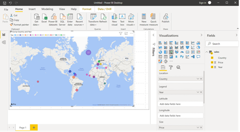
After loading the data, we can build the report. We will use the Map visual, where we populate the properties using data from the sales table as follows:

• Location: country
• Legend: year
• Size: price

This configuration renders the visual below:

We can now publish the report in our workspace. We save the report locally and then click the Publish button in the top pane. The Power BI desktop asks us to sign in to our account then choose the destination workspace. We pick the one we created earlier (SynapseDemo):

After a short while, the report publishes, and we can go back to Azure Synapse Studio. We will not need to refresh the Studio, so the report becomes visible under the Develop tab (Power BI). When we click the report, it renders the same way as in Power BI Desktop and the Power BI service:

We can also modify the report directly from Azure Synapse Studio. This capability enables us to adjust the source data and immediately see the changes we make without leaving our environment.

Summary

This article explored Azure Synapse Studio features for querying, filtering, and aggregating data with almost no code. To do this, we only made minor changes to automatically-generated code blocks, making the Azure Synapse Studio an excellent tool for data scientists who may not specialize in developing code.

We learned that Azure Synapse Studio easily synchronizes with other Azure services (like SQL pools, Spark pools, and Azure Cosmos DB) and Microsoft applications (like Power BI). These integrations enable us to incorporate data science and machine learning pipelines into existing applications to get insights from all our data without slowing our applications. In the SQL API of Azure Cosmos DB, we would need to migrate existing containers to support analytical storage.

We worked with small datasets to reduce the cost when writing data to Azure Cosmos DB along this journey. However, Azure Synapse can easily import millions of rows within a few minutes. For instance, the official Azure Synapse’s datasets can load two million rows of NYC Taxi data to a dedicated SQL pool within one minute. You can use the tools and techniques in this article series to analyze your large datasets.

Check the GitHub repo to find more code samples.

Want even more Azure Synapse training? Check out Microsoft’s Hands-on Training Series for Azure Synapse Analytics. You can start your first Synapse workspace, build code-free ETL pipelines, natively connect to Power BI, connect and process streaming data, and use serverless and dedicated query options.