Step-by-Step Guide to Implement Machine Learning V - Support Vector Machine

Ryukkkk

Rate me:

5.00/5 (3 votes)

14 May 2019CPOL4 min read

5.5K

Easy to implement machine learning

This article is an entry in our Machine Learning and Artificial Intelligence Challenge. Articles in this sub-section are not required to be full articles so care should be taken when voting.

Introduction

Support Vector Machine(SVM) is a classifier based on the max margin in feature space. The learning strategy of SVM is to make the margin max, which can be transformed into a convex quadratic programming problem. Before learning the algorithm of SVM, let me introduce some terms.

Functional margin is defined as: For a given training set T, and hyper-plane(w,b), the functional margin between the hyper-plane (w,b) and the sample(xi, yi) is:

$\hat{\gamma}_{i}=y_{i}\left(w\cdot x+b\right)$

The functional margin between hyper-plane (w,b) and the training set T is the minimum of $\hat{\gamma}_{i}$

$\hat{\gamma}=\min\limits_{i=1,...,N} \hat{\gamma}_{i}$

Functional margin indicates the confidence level of the classification results. If the hyper-parameters (w,b) change in proportion, for example, change (w,b) into (2w,2b). Though the hyper-plane hasn't changed, the functional margin expend doubles. Thus, we apply some contrains on w to make the hyper-plane definitized , such as normalization ||w|| = 1. Then, the margin is called geometric margin: For a given training set T, and hyper-plane(w,b), the functional margin between the hyper-plane (w,b) and the sample(xi, yi) is:

${\gamma}_{i}=y_{i}\left(\frac{w}{||w||}\cdot x_{i}+\frac{b}{||w||}\right)$

Similarly, the geometric margin between hyper-plane (w,b) and the training set T is the minimum of ${\gamma}_{i}$

${\gamma}=\min\limits_{i=1,...,N} {\gamma}_{i}$

Now, we can conclude the relationship between functional margin and geometric margin:

$\gamma_{i}=\frac{\hat{\gamma_{i}}}{||w||}$

$\gamma=\frac{\hat{\gamma}}{||w||}$

SVM Model

The SVM model consists of optimization problem, optimization algorithm and classify.

Optimization Problem

When the dataset is linearly separable, the supports vectors are the samples which are nearest to the hyper-plane as shown below.

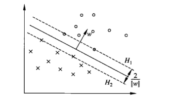
The samples on H1 and H2 are the support vectors.The distance between H1 and H2 is called hard margin. Then, the optimization problem of SVM is:

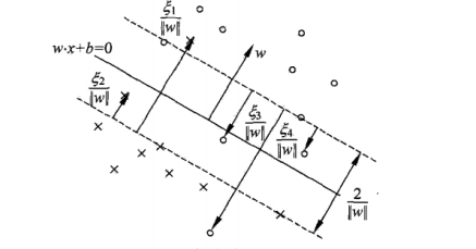
$\min\limits_{w,b}\ \frac{1}{2}||w||^{2}\\ s.t.\ y_{i}\left(w\cdot x+b\right)-1\geq 0,\ i=1,2,...,N$

When the dataset is not linearly separable, some samples in the training set don't satisfy the condition that the functional margin is larger than or equal to 1. To solve the problem, we add a slack variable $\xi_{i}\geq0$ for each sample (xi, yi). Then, the constraint is:

$y_{i}\left(w\cdot x+b\right)\geq 1-\xi_{i}$

Meanwhile, add a cost for each slack variable. The target function is:

$\frac{1}{2}||w||^{2}+C\sum_{i=1}^{N}\xi_{i}$

where C is the penalty coefficient. When C is large, the punishment of misclassification will be increased, whereas the punishment of misclassification will be reduced. Then, the optimization problem of SVM is:

$\min\limits_{w,b}\ \frac{1}{2}||w||^{2}+C\sum_{i=1}^{N}\xi_{i}\\ s.t.\ y_{i}\left(w\cdot x+b\right)\geq 1-\xi_{i},\ i=1,2,...,N\\ \xi_{i}\geq0,\ i=1,2,...,N$

The support vectors are on the border of margin or between the border and the hyper-plane as shown below. In this case, the margin is called soft margin.

It needs to apply kernel trick to transform the data from original space into feature space when the dataset is not linearly separable. The function for kernel trick is called kernel function, which is defined as:

$K\left(x,z\right)=\phi\left(x\right)\cdot \phi\left(z\right)$

where $\phi\left(x\right)$ is a mapping from input space to feature space, namely,

$\phi\left(x\right):\chi\rightarrow\mathcal{H}$

The code of kernel trick is shown below:

Python

def kernelTransformation(self, data, sample, kernel):
        sample_num, feature_dim = np.shape(data)
        K = np.zeros([sample_num])
        if kernel == "linear":  # linear function
            K = np.dot(data, sample.T)
        elif kernel == "poly":  # polynomial function
            K = (np.dot(data, sample.T) + self.c) ** self.n
        elif kernel == "sigmoid":  # sigmoid function
            K = np.tanh(self.g * np.dot(data, sample.T) + self.c)
        elif kernel == "rbf":  # Gaussian function
            for i in range(sample_num):
                delta = data[i, :] - sample
                K[i] = np.dot(delta, delta.T)
            K = np.exp(-self.g * K)
        else:
            raise NameError('Unrecognized kernel function')
        return K

After applying kernel trick, the optimization problem of SVM is:

$\min\limits_{\alpha}\ \ \frac{1}{2}\sum_{i=1}^{N}\sum_{j=1}^{N}\alpha_{i}\alpha_{j}y_{i}y_{j}K\left(x_{i},y_{j}\right)-\sum_{i=1}^{N}\alpha_{i}\\s.t.\ \ \sum_{i=1}^{N}\alpha_{i}y_{i}=0\\ 0\leq\alpha_{i}\leq C,i=1,2,...,N$

where $\alpha_{i}$ is the Lagrange factor.

Optimization Algorithm

It is feasible to solve the SVM optimization problem with traditional convex quadratic programming algorithms. However, when the training set is large, the algorithms will take a long time. To solve the problem, Platt proposed an efficient algorithm called Sequential Minimal Optimization (SMO).

SMO is a kind of heuristic algorithm. When all the variables follow the KKT condition, the optimization problem is solved. Else, choose two variables and fix other variables and construct a convex quadratic programming problem with the two variables. The problem has two variables: one chooses the alpha which violated KKT conditions, the other is determined by the constraints. Denote, the $\alpha_{1,}\alpha_{2}$ are the variables, fix $\alpha_{3},\alpha_{4},...,\alpha_{N}$ . Thus, $\alpha_{1}$ is calculated by:

$\alpha_{1}=-y_{1}\sum_{i=2}^{N}\alpha_{i}y_{i}$

If $\alpha_{2}$ is determined , $\alpha_{1}$ is determined accordingly. In each iteration of SMO, two variables are updated till the problem solved. Then, the optimization problem of SVM is:

$\min\limits_{\alpha_{1},\alpha_{2}} W\left(\alpha_{1},\alpha_{2}\right)=\frac{1}{2}K_{11}\alpha_{1}^{2}+\frac{1}{2}K_{22}\alpha_{2}^{2}+y_{1}y_{2}K_{12}\alpha_{1}\alpha_{2}-\\\left(\alpha_{1}+\alpha_{2}\right)+y_{1}\alpha_{1}\sum_{i=3}^{N}y_{i}\alpha_{i}K_{i1}+y_{2}\alpha_{2}\sum_{i=3}^{N}y_{i}\alpha_{i}K_{i2}\\s.t.\ \ \ \alpha_{1}y_{1}+\alpha_{2}y_{2}=-\sum_{i=3}^{N}y_{i}\alpha_{i}\\ 0\leq\alpha_{i}\leq C,i=1,2$

When there is only two variable, it is a simple quadratic programming problem, as shown below:

Because the constraint is:

$\alpha_{1}y_{1}+\alpha_{2}y_{2}=-\sum_{i=3}^{N}y_{i}\alpha_{i} = k$

when $y_{1}=y_{2}$ , $\alpha_{1}+\alpha_{2}=k$

when $y_{1}\ne y_{2}$ , because $y_{1},y_{2}\in\left\{1，-1\right\}$ , $\alpha_{1}-\alpha_{2}=k$ .

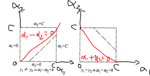
The optimized value $\alpha_{2}^{new}$ follows:

$L\leq\alpha_{2}^{new}\leq H$

where L and H are the lower bound and upper bound of the diagonal line, which is calculated by:

$L,H=\left\{ \begin{aligned} L= max\left(0, \alpha_{2}^{old}-\alpha_{1}^{old}\right),H= min\left(C,C+ \alpha_{2}^{old}-\alpha_{1}^{old}\right) if\ y_{1}\ne y_{2} \\ L= max\left(0, \alpha_{2}^{old}+\alpha_{1}^{old}-C\right),H= min\left(C,\alpha_{2}^{old}+\alpha_{1}^{old}\right) if\ y_{1}= y_{2} \\ \end{aligned} \right.$

The uncutting optimized value $\alpha_{2}^{new,unc}$ follows:

$\alpha_{2}^{new,unc}=\alpha_{2}^{old}+\frac{y_{2}\left(E_{1}-E{2}\right)}{\eta}$

where E₁and E₂ are the difference between the prediction value g(x) and the real value. g(x) is defined as:

$g\left(x\right)=\sum_{i=1}^{N}\alpha_{i}y_{i}K\left(x_{i},x\right)+b$

$\eta=K_{11}+K_{22}-2K_{12}$

So far, we get feasible solutions for $\alpha_{1,}\alpha_{2}$ :

$\alpha_{2}^{new}=\left\{\begin{aligned} &H,&\alpha_{2}^{new,unc}>H\\ &\alpha_{2}^{new,unc},&L\leq\alpha_{2}^{new,unc}\leq H\\ &L,&\alpha_{2}^{new,unc}<L\end{aligned}\right.$

$\alpha_{1}^{new}=\alpha_{1}^{old}+y_{1}y_{2}\left(\alpha_{2}^{old}-\alpha_{2}^{new}\right)$

There are two loops in SMO, namely, outside loop and inner loop.

In the outside loop, choose the alpha which violated KKT conditions, namely,

$\alpha_{i}=0\Leftrightarrow y_{i}g\left(x_{i}\right)\geq1\\ 0<\alpha_{i}<C\Leftrightarrow y_{i}g\left(x_{i}\right)=1\\ \alpha_{i}=C\Leftrightarrow y_{i}g\left(x_{i}\right)\leq1$

First, search the samples follow $0<\alpha_{i}<C$ .If all the samples follow the condition, search the whole dataset.

In the inner loop, first search the $\alpha_{2}$ which make $\left|E_{1}-E_{2}\right|$ maximum. If the chosen $\alpha_{2}$ doesn't decrease enough, first search the samples on the margin border. If the chosen $\alpha_{2}$ decreases enough, stop search. Else, search the whole dataset. If we can find a feasible $\alpha_{2}$ after searching the whole dataset, we will choose a new $\alpha_{1}$ .

In each iteration, we updated b by:

$b_{1}^{new}=-E_{1}-y_{1}K_{11}\left(\alpha_{1}^{new}-\alpha_{1}^{old}\right)-y_{2}K_{21}\left(\alpha_{2}^{new}-\alpha_{2}^{old}\right)+b^{old}$

$b_{2}^{new}=-E_{2}-y_{1}K_{12}\left(\alpha_{1}^{new}-\alpha_{1}^{old}\right)-y_{2}K_{22}\left(\alpha_{2}^{new}-\alpha_{2}^{old}\right)+b^{old}$

$b=\left\{\begin{aligned} &b_{1}^{new},&if\ 0<\alpha_{1}^{new}\\ &b_{2}^{new},&if\ 0<\alpha_{2}^{new}\\ &\frac{b_{1}^{new}+b_{2}^{new}}{2},&else\end{aligned}\right.$

For convenience, we have to store the value of $E_{i}$ , which is calculated by:

$E_{i}^{new}=\sum_{s}y_{j}\alpha_{j}K\left(x_{i},y_{j}\right)+b^{new}-y_{i}$

The search and update code is shown below:

Python

def innerLoop(self, i):
        Ei = self.calculateErrors(i)
        if self.checkKKT(i):

            j, Ej = self.selectAplha2(i, Ei)          # select alpha2 according to alpha1

            # copy alpha1 and alpha2
            old_alpha1 = self.alphas[i]
            old_alpha2 = self.alphas[j]

            # determine the range of alpha2 L and H      in page of 126
            # if y1 != y2    L = max(0, old_alpha2 - old_alpha1), 
                             H = min(C, C + old_alpha2 - old_alpha1)
            # if y1 == y2    L = max(0, old_alpha2 + old_alpha1 - C), 
                             H = min(C, old_alpha2 + old_alpha1)
            if self.train_label[i] != self.train_label[j]:
                L = max(0, old_alpha2 - old_alpha1)
                H = min(self.C, self.C + old_alpha2 - old_alpha1)
            else:
                L = max(0, old_alpha2 + old_alpha1 - self.C)
                H = min(self.C, old_alpha2 + old_alpha2)

            if L == H:
                # print("L == H")
                return 0

            # calculate eta in page of 127 Eq.(7.107)
            # eta = K11 + K22 - 2K12
            K11 = self.K[i, i]
            K12 = self.K[i, j]
            K21 = self.K[j, i]
            K22 = self.K[j, j]
            eta = K11 + K22 - 2 * K12
            if eta <= 0:
                # print("eta <= 0")
                return 0

            # update alpha2 and its error in page of 127 Eq.(7.106) and Eq.(7.108)
            self.alphas[j] = old_alpha2 + self.train_label[j]*(Ei - Ej)/eta
            self.alphas[j] = self.updateAlpha2(self.alphas[j], L, H)
            new_alphas2 = self.alphas[j]
            self.upadateError(j)


            # update the alpha1 and its error in page of 127 Eq.(7.109)
            # new_alpha1 = old_alpha1 + y1y2(old_alpha2 - new_alpha2)
            new_alphas1 = old_alpha1 + self.train_label[i] * 
                          self.train_label[j] * (old_alpha2 - new_alphas2)
            self.alphas[i] = new_alphas1
            self.upadateError(i)

            # determine b in page of 130 Eq.(7.115) and Eq.(7.116)
            # new_b1 = -E1 - y1K11(new_alpha1 - old_alpha1) - 
                             y2K21(new_alpha2 - old_alpha2) + old_b
            # new_b2 = -E2 - y1K12(new_alpha1 - old_alpha1) - 
                             y2K22(new_alpha2 - old_alpha2) + old_b
            b1 = - Ei - self.train_label[i] * K11 * (old_alpha1 - self.alphas[i]) - 
                        self.train_label[j] * K21 * (old_alpha2 - self.alphas[j]) + self.b
            b2 = - Ej - self.train_label[i] * K12 * (old_alpha1 - self.alphas[i]) - 
                        self.train_label[j] * K22 * (old_alpha2 - self.alphas[j]) + self.b
            if (self.alphas[i] > 0) and (self.alphas[i] < self.C):
                self.b = b1
            elif (self.alphas[j] > 0) and (self.alphas[j] < self.C):
                self.b = b2
            else:
                self.b = (b1 + b2)/2.0

            return 1
        else:
            return 0

Classify

We can make a prediction using the optimized parameters, which is given by:

$f\left(x\right)=sign\left(\sum_{i=1}^{N}\alpha_{i}^{*}y_{i}K\left(x,x_{i}\right)+b^{*}\right)$

Python

for i in range(test_num):
    kernel_data = self.kernelTransformation(support_vectors, test_data[i, :], self.kernel)
    probability[i] = np.dot(kernel_data.T, np.multiply
                     (support_vectors_label, support_vectors_alphas)) + self.b
    if probability[i] > 0:
        prediction[i] = 1
    else:
        prediction[i] = -1

Conclusion and Analysis

SVM is a more complex algorithm than previous algorithms. In this article, we simplify the search process to make it a bit more easy to understand. Finally, let's compare our SVM with the SVM in Sklearn and the detection performance is displayed below:

The detection performance is a little worse than the sklearn's , which is because the SMO in our SVM is simpler than sklearn's.

The related code and dataset in this article can be found in MachineLearning.

License

This article, along with any associated source code and files, is licensed under The Code Project Open License (CPOL)

Written By

Ryukkkk

Engineer

Germany

Ryuk is interested in Machine Learning/Signal Processing/VoIP.

Step-by-Step Guide to Implement Machine Learning V - Support Vector Machine

Introduction

SVM Model

Optimization Problem

Optimization Algorithm

Classify

Conclusion and Analysis

License

Comments and Discussions