Understanding Long Short-Term Memory Networks (LSTMs)

Remember how in the previous article we’ve said that we can predict text and make speech recognition work so well with Recurrent Neural Networks? The truth is that all the big accomplishments that we assigned to RNNs in the previous article are actually achieved using special kind of RNNs – Long Short-Terms Memory Units (LSTMs).

This upgraded version of RNNs solved some of the problems that these networks usually have. Since the concept of RNNs, like most of the concepts in this field, has been around for a while, scientists in the 90s noticed some obstacles in using it. There are two major problems that standard RNNs have: Long-Term Dependencies problem and Vanishing-Exploding Gradient problem.

Long-Term Dependencies Problem

We’ve just mentioned the subject of Long-Term Dependencies in the previous article, so let’s get more into details here. One of the perks of using RNNs is that we can connect previous information to the present task and based on that, make certain predictions. For example, we can try to predict what will be the next word in the certain sentence based on the previous word from the sentence. And RNNs are great for these kind of tasks when we need to look only at the previous information to perform a certain task. However, that is really the case.

Take that example of text prediction in language modeling. Sometimes, we can predict the next word in the text based on the previous one, but more often we need more information than just the previous word. We need context, we need more words from the sentence. RNNs are not good with this. The more previous states we need for our prediction, the bigger problem this represents for standard RNN.

Vanishing-Exploding Gradient Problem

As you probably know, gradient expresses the change in the weights with regards to change in the error. So, if we don’t know the gradient, we cannot update weights in a proper direction, and reduce the error. The problem that we face in every Artificial Neural Network is that if the gradient is vanishingly small, it will prevent the weights from changing their value. For example, when you apply sigmoid function multiple times, data gets flattened until it has no detectable slope. The data is flattened until, for large stretches, it has no detectable slope. The same thing happens to the gradient as it passes through many layers of a neural network.

In RNNs, this problem is bigger due to the fact that during the learning process of Recurrent Neural Networks, we update them “trough time”. We use Backpropagation Through Time, and this process introduces even more multiplications and operations than regular backpropagation. Of course, this gradient problem can go the other way. The gradient can become progressively bigger and cause butterfly effect in the RNN, so-called exploding gradient problem.

LSTM Architecture

In order to solve obstacles that Recurrent Neural Networks face, Hochreiter & Schmidhuber (1997) came up with the concept of Long Short-Term Memory Networks. They are working very well on the large range of problems and are quite popular now. The structure is similar to the structure of standard RNN, meaning they feed output information back to the input, but these networks don’t struggle with problems that standard RNNs do. In their architecture, they have implemented a mechanism for remembering long dependencies.

If we observe an unfolded representation of the standard RNN, we consider it to be a chain of repeating structure. This structure is usually pretty simple, such as the single tahn layer.

LSTMs even though they follow the similar principle, have considerably more complicated architecture. Instead of a single layer, they usually have four and they have more operations regarding those four levels. Example of single LSTM unit’s structure can be seen in the image below:

Here is the legend for elements from this graph:

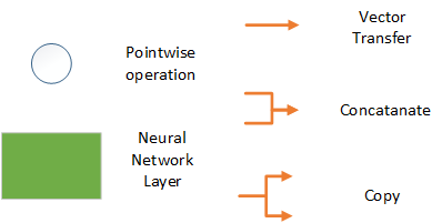
As you can see in the image, we have four network layers. One layer is using the tahn function and two layers are using the sigmoid function. Also, we are having some pointwise operations and regular operations on the vectors, like concatenation. We will explore this in more detail in the next chapter.

The important thing to notice however is the upper data stream marked with the letter C. This data stream is holding information outside the normal flow of the Recurrent Neural Network and is known as the cell state. Essentially data transferred using the cell state is acting much like data in computer’s memory because data can be stored in this cell state or read from it. LSTM Cell decides what information will be added to the cell states using analog mechanisms called gates.

These gates are implemented using element-wise multiplications by sigmoids (range 0-1). They are similar to the neural network’s nodes. Based on the strength input signal, they pass that information to the cell state or block it. For this purpose, they have their own set of weights that is maintained during the learning process. This means that LSTM cells are trained to filter certain data and to preserve the error, that later can be used in backpropagation. Using this mechanism, LSMT networks are able to learn over many time steps.

LSTMs Process

LSTM cells operate in few steps:

1. Forget unnecessary information from the cell state
2. Add information to the cell state
3. Calculate the output

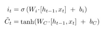
First sigmoid layer in LSTM cell is called forget gate level. Using this layer/gate, the LSTM cell is deciding how important is the previous state in the cell Ct-1 is and we are deciding what will be removed. Since we are using the sigmoid function, that ranges from 0 to 1, so data can be completely removed, partially removed, or completely preserved. This decision is made by looking at previous state Ht-1 and current input Xt. Using this information and sigmoid level, LSTM cell generates a number between 0 and 1 for each number in the cell state Ct−1:

When unnecessary information is removed, LSTM cell decides which data is going to be added to the cell state. This is done by the combination of second sigmoid and tahn levels. Firstly, second sigmoid layer, also known as input gate layer, decides which values in the cell state will be updated (output – i) and then tahn layer creates a vector of new candidate values that could be added to the cell state (outputs ~Ct).

Effectively, using this information, the new value of the cell state is calculated – Ct.

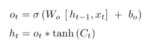
The last step we need to do is to calculate the output of LSTM cell. That is done using third sigmoid level and additional tahn filter. The output value is based on values in the cell state, but it is also filtered by sigmoid layer. Basically, sigmoid layer decides which parts of the cell state are going to affect the output value. Then we put cell state value through the tahn filter (pushes all values between -1 and 1) and multiply it by the output of the third sigmoid level.

Conclusion

This upgraded version of RNN is actually what made these type of networks so popular. They achieve tremendous results because of their ability to preserve data through time. The only shortcoming of these networks is that training is quite time-consuming, and require a lot of resources. As you can imagine, training this complex structure cannot be cheap. Apart from that, they are one of the best choices when it comes to problems that require processing sequences of data.

Thanks for reading!