Rubber Duckies in Dynamical Systems

• Download scripts - 170.6 KB

Introduction

It was about 5 years ago that I revealed, here in the pages of Code Project, my discovery of The Bad Mandelbrot Set. Only, it sort of turned out that other people had tripped over the same mistake I made and even named the Bad Mandelbrot Set as the Tricorn or Mandelbar Set. Well, this time, I'm sure I've found a few things that are completely new and previously unknown.

If you can cite any previously published articles or references that disprove my claims of originality, I (we?) would like to see them. But please, only reference material we can see publicly without cost. For-pay journals and reviews are great but they don't exactly fit with Code Project's evident "information should be freely shared" principle.

I would warn the Python scripts here do require a bit of speed. I have tried them on a Raspberry Pi 4, and that seems to be the low end of enjoyable performance for many of these demonstrations.

But Before That, A Brief Bit of Basic Background

The simplest dynamical system that does any good is the one that approximates a circle. For any point in the 2D plane not at the origin, if you move the point a bit at a right angle to the radial vector from the origin to the point in either the clockwise (CW) or counter-clockwise (CCW) direction, you will start to make a circle. The move is tangential to the circle you are approximating. All you have to do is re-evaluate what is tangential once the point has moved a bit. This diagram shows a point, (x, y), in the first quadrant, but the math holds for any quadrant and any angle in it.

Say we add 5% of the clockwise tangent to the point (x, y). The equations that would give us the new x and y are:

x += .05 * y
y -= .05 * x

What is not immediately obvious is that the first equation needs to be evaluated for the new value of x before the second equation is evaluated using that new x value. I call this property or attribute of this dynamical system "ordered". There are other meanings for "ordered dynamical system" but in this article, ordered means the 'map' of the dynamical system (the set of dimension equations evaluated for the new point) is evaluated dimension equation by dimension equation. The alternative is "discrete". This is what that map would look like for a circle-approximating dynamical system with discrete evaluation:

temp = x
x += .05 * y
y -= .05 * temp

The term "discrete" is as used here. Full map evaluations occur at discrete instances (of time) using a copy of the current point. There is no using intermediate new dimension values to calculate other new dimension values during the map evaluation.

Why does the circle's dynamical system need to be ordered? This diagram helps show that the discrete evaluation values miss the circle's curvature significantly whereas evaluating the ordered new y from a slightly bigger new x gets us closer to the circle. This error is offset on the opposite side of the ordered circle whereas the discrete circle wanders too much to stay on track.

Also, if we use a smaller delta (say 1% instead of 5%), the error wobble is reduced. In the limit, delta goes to zero and these difference equations become differential equations where the error wobble also goes to zero.

What about the complex plan? Is there a circle-approximating dynamical system here and is it ordered or discrete? Please try the two scripts from the download: circOrbit.py and circOrbitComplex.py to find out.

Short of going to the limit, maybe we could resolve the difference between the Ordered and Discrete circle dynamical systems by handling the map a little differently. What if, instead of evaluating the next step at delta (.05), we evaluated the map at half of delta and then used this intermediate midpoint's values to make a full delta step? That is, for the ordered map, instead of,

x = x + delta * y
y = y - delta * x

we did:

x2 = x + .5*delta * y
y2 = y - .5*delta * x2

and then did:

x = x + delta * y2
y = y - delta * x2

There is a similar discrete mapping that uses midpoints. Midpointing helps tremendously. The ordered map circle has no visible wobble, and the discrete map circle spirals outward very slowly. You can run circOrbitMidpoint.py to see this. Click "Using Full steps." to change to "Using Midpoints." and click "Start" or "New Start". See the pretty circle.

Now click "Using Ordered map" so "Using Discrete map" is selected. A sleep delay is used to keep the animation slow enough to see the circle being generated. Click the "Speed up" button to prevent delays ("Go slow" in the diagram). You will see the circle expand quickly. It will stop when the new point reaches a maximum distance from the origin).

So we've fixed the wobble in one mapping and improved the other. Can we do better? Maybe we just need more accurate estimates. Instead of using just one midpoint, we could use one half step estimate and another half step estimate based on the values of the first half step and a full step estimate based on the second half step's values. Then we could weight the current point, the two half step estimates and the full step by 1/6, 2/6, 2/6, and 1/6 to come up with a really, really good next point. Please check the step() function in circOrbitRK4.py to see the details of this mapping.

This time, we've improved both mappings, but now speeding up the "Using Ordered map", "Using Midpoints." dynamical system shows a slowly contracting cirle while the "Using Discrete map", "Using Midpoints." circle appears to be stable (actually, it contracts too, vey slowly — Try minimizing the Tk window for many seconds when 'delta is 0.2' or several minutes when 'delta is 0.1'). You can't win with extra accuracy. You may want to examine circOrbitIntegrate.py. It allows using an RK3-ish estimator and a one-third step integrator to make steps. Depending on the combination of controls, you will find expanding dynamical systems or ones that spiral inward.

The point I am trying to make is that it's as worthwhile to study "Ordered" (my meaning) dynamical systems as it is to study classic 'discrete' ones. The only completely stable approximators here are the original Ordered mapping and its midpointed, de-wobbled improvement. And frankly, to me, only the original has a natural, simple beauty in its map.

More than Just a Circle

Moving beyond a circle, what we really need is something that will whoosh and swoop around with a strange but stable behavior. Please try the SA2dDuffing.py script. This attractor relies on both a "double-well" potential to attract a point to two distinct minima, (like the single minimum tangential-force spot at the origin in our circles above), plus a driver to get some strangeness going on as our point tries to orbit one or the other minima.

The most tractable description of the Duffing Equation I've found is by Dr. A. Peter Young from UCSC. He couches his class examples in Mathematica (still not free from what I can see) but the descriptions and explanations are very good. Dr. Young chose to use a cosine value of 1.4*t whereas SA2dDuffing.py uses 1*t. In either case, the force definition used in the Duffing Equation turns out to be more than a little important.

You can set a value for a which is a dampening factor for the driver and b which gives the driver's amplitude. A negative dampening factor makes an amplifier which leads to explosive growth in the orbit. An amplitude that is too small does not give the driver enough oomph (to use the scientific term) to send the point from one well to the other. With a dampening factor of 0.2, the critical amplitude is around 0.27.

Without enough oomph, the orbit will eventually settle to a limit cycle around one of the minima. Even with adequate driving, the orbit can settle to a limit cycle around both minima. While "Using Plus Map" or "Using Minus Map" and "Using Ordered Map", try setting a == .3 and b == .365. The orbit will settle to one like the following. Can you tell if this is the '+' map, or '-' map?

For this attractor, there doesn't seem to be any great difference between using and Ordered or Discrete map. For the Discrete map, the control point (.3, .385) is similar to the Ordered map's (.3, .365) but only one minima is double looped. "New Point" seems to affect which minima is double looped as much as using the + or - map.

Well, strange attractors and limit cycles in two dimensions are all great and everything but what about 3D?

And Now for Something Completely New and Previously Undisclosed

I found the limit cycles in LCbball.py and LCtumble.py in the 90's. LCbball.py is named because the trajectory reminded me of the seam of a baseball. LCtumble.py is named because I thought of a rag doll following this trajectory head first — it would tumble.

Imagine a tilted globe. LCtumble.py marks out a trajectory at the equator moving east 90 degrees, then up to the North Pole, turning 90 degress right, then back to the equator, then west 90 degrees until it is nearly at the position after the first move, then down to the South Pole, 90 degree left turn and back to the equator, then repeat the last six moves only switch poles. This is the magnetic tunnel limit cycle I use in my own fusion reactor. Both scripts have '<-' and '->' buttons to turn the limit cycle left or right for viewing. Click "Clear View" to see the limit cycle retraced. LCtumbleMinus.py is another less interesting limit cycle. All three use Ordered maps.

Putting LCs to Work in the 3D World

Why implement all this stuff in Python and TkInter? Because anyone can easily get Python which usually includes a tkinter library (with proviso for MacOS). Why use a non-JITted runtime environment? Because we don't really need the speed, and where we do, I've tried to offer workarounds. BTW, I've also tried to accommodate dead Python 2. But then, why not use pyopengltk or other OpenGL framework? There you've got me. I wanted to unhide what OpenGL does. I developed knownWorld.py to see if I could understand and make a world viewer of my own using well-known maths.

We set up our limit cycles or strange attractors for viewing at the origin of the world. We have a camera that always 'looks at' the origin. And we move the camera about to view our thingies. We also make a perspective projection of the viewed thingy for realism.

What if we used a simple 2D circle orbiter, or the bball LC, or the tumble LC to automatically move the camera to look at thingies from different angles? wellKnown3dAttractors.py does this. Many of these attractors were taken with some modifications from parameters on this page and from here.

All good, but what about this "rubber ducky" business?

Now for Something Totally New and Previously Unseen

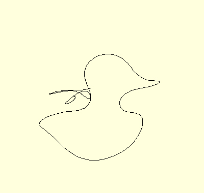
I discovered the Barnes attractors this year. ('Barnes' attractor? Hey, I'm an old guy now. I've got to grab for what fame I can while I still am.) Yes, so you will probably notice 'barnes' showing up in many download file names. Let's take a look at barnes3dCubic.py. This attractor has the tendency of occasionally making projected outlines of rubber duckies, like that seen at the start of this article. Here is another screen shot of this script with an embedded ducky:

Surprise, this attractor requires an Ordered map. "Start" the attractor. Once it has been ordering about for a few seconds, try clicking the "Ordered Map" button to use the "Discrete Map". The trajectory will continue for a while but sooner or later, it will blow up.

This attractor has seven repulsive fixed points. If you look at the step() function in barnes3dCubic.py, you can almost guess their locations. First, the origin itself is a fixed point. If all three dimension values are zero, each delta amount in the map equations will be zero.

p.x += .05*(p.z + p.y * p.x * p.x - p.z * p.z * p.z)
p.y += .05*(p.x + p.z * p.y * p.y - p.x * p.x * p.x)
p.z += .05*(p.y + p.x * p.z * p.z - p.y * p.y * p.y)

Now imagine just one dimension is +1.0 or -1.0 and the other two are zero. Since each map equation contains dimension - dimension^^3 terms (sound familiar?), the dimension that is +1.0 or -1.0 will contribute zero to the delta amount with the other term being a product of zeros. The other two map equations will have all-zero terms, so these points stay fixed. They form a veritable cage of repulsion. So why should any point stick around? Where's the attraction, strange or otherwise?

The trick is the +1.0 / -1.0 fixed points are VERY twisty. If you run barnes3dCubicAttractorField.py and click "Show", a circular area of the attractor field will be shown. Notice the little swirls at (0,-1,0) and (0,+1,0). No, the axes and coordinates are not marked, but you should be able to discern where these coordinates are. You have to rotate the "x==0 dial" right to a longitudinal viewing angle of about -30 degrees to see the (0,0,-1) and (0,0,+1) swirls clearly. There are other "dials" that can be displayed. For performance, the script limits display to a maximum of three dials. Also, if you have the sortedcontainers module available, there is a "Do sorting" switch that can help when two or three dials are displayed (checked).

The attractor is so chaotic, it's hard to get a good idea of its overall shape. The attractor field script shows circular dials of the field but not the actual attractor. Let's take a look at barnes3dCubicBasin.py. It shows the basin of this attractor in blue. The basin is an envelope-like enclosure. Trajectories with initial points chosen inside the basin will settle to within the attractor hull. If you have sortedcontainers, the maxima of the attractor's hull is shown in a different color. Since the basin and hull are so far apart, this attractor is very stable.

Is that a ruby-throated hummingbird or a strange, warped little ducky? Even when single random map equations are successively chosen with no back-to-back repeats, DuckyOnCrack.py, or delta is sporadically switched between '+' and '-' for each full mapping, FickleDuck.py, this attractor remains chaotic, if not deterministic, for quite a while.

The Good, the Bad, and the Ugly

Besides stability, what's so good about the Barnes 3D Cubic attractor? Two things really. First, delta's can be consistently added or always subtracted. Run the barnes3dCubic.py script again and click "Start". Now try clicking the "+= δ Map" button so "-= δ Map" is selected. You will see the point's trajectory reverse, although not exactly. It's the same attractor but maybe the "anti" version.

Second, the mapping itself can be in any of six orders: xyz, yzx, zxy, xzy, zyx, or yxz. 3! orderings for 3 dimensions. Visually all six are indistinguishable.

And the bad part? The bad is that this attractor is a bit ugly (surprising considering where it came from). While running barnes3dCubic.py, click the "Show endpoints" button and keep clicking "More lines" until your finger gets tired. There's no pattern to be seen in the points displayed. This is because the Barnes 3D Cubic attractor does not form a manifold, or dare we say brane. Or maybe it is just a very narrow, tangled one, like the tightly-curled ribbon on some gift. Some of the graceful well-known 3D attractors in wellKnown3dAttractors.py form large sweeping manifolds, like the wide bows on other gifts. This article on Chaos topology discusses "Weakly dissipative 3D systems". I believe 'dissipative' is a measure of how quickly a chaotic dynamical system settles to a, possibly many-"branched", manifold. Like the 1984 Lorenz 3D weakly dissipative system, the Barnes 3D Cubic attractor ain't doin' no dissipatin'.

The salient property of a manifold is that it can divide the space of the next higher dimension that can contain the manifold in two, i.e.,: the manifold has sides.

For two vectors not pointing in the same direction, you can take their cross product and get a vector that is at right angles to both. We can do this with two consecutive line segments in an attractor's trajectory and color the leading segment based on this cross product. For a small region of arcs in the ribbon of a manifolding attractor, nearby arcs should have a similar curvature (cross products pointing in the same direction, same color). Also nearby arcs should not be skew (different cross product, different color), except where branching or folding is occurring. Otherwise there should be no off-color, "piercing" arcs intervening. If the Barnes 3D Cubic attractor makes a manifold, it must be a very narrow and infinitely tangled one. Please try rosslerBarnesManifolding.py. The Rossler side should look not-ugly while the Barnes side should look... colorful.

When sortedcontainers is around, you can "Sort" the display when you choose or you can change "Views unsorted" to "Sorting new views" to sort when moving the camera or changing scale. This is the one demo where a JITted, hadware-assisted, OpenGL shader would have helped. Depth sorting per new line segment in a straight Tk display is too slow.

For an improvement, our fellow Code Project member, Samuel Teixeira, provided the 5-star OpenGL in Python with TKinter in 2016. Perhaps Jon Wright's 2018 pyopengltk is partly based on that. There are other platforms such as three.js and OpenTK that suggest themselves for Javascript and C# devotees.

I hope to update with a better image in the future, but for now, I include this taken from wellKnown3dAttractors.py selecting the "Barnes" attractor using a high line count and viewing from a high polar angle. Notice the predominant red, green, and blue swirls near the +1.0/-1.0 fixed points. And that they swirl in the same direction (curvature) on both sides of the origin.

Tossing the Kitchen Sink at the Entire Pig
While it Rings and Reports Wrongdoing

There are a few more things I'd like to point out about the Barnes 3D Cubic attractor. If you have a display that is at least HD (1920 x 1080), you can try running the rather large barnes3dCubic3pts12ways.py.

Precision

I was a little amazed this attractor remains chaotic with only 3 digits of precision. Before "Start" if you click "▲" on the "Signif. Digits:" Spinbox, the attractor will use three decimal digits of significance. The Spinbox wraps from 50 max back down to 3. When you click "Start", you should see three trajectory points start from the same position: One in black, a second in red, and the third spring green. They wander apart as is their wont because, well, because they are strange. When you "Pause" running, the trajectory points' end values are displayed with three significant digits.

Please notice the Entry box under "Sep▼". It shows the last maximum separation between the three trajectory points whenever the maximum exceeds 0.25 units. The points can only get so far apart because they share the same origin. Also note the "Arm Pause" button that is discussed later.

Deterministic Trajectories

This is really a property of all "solvable" dynamical systems. What it means is that starting the system at the same initial point will always repeat the exact same trajectory from start to the end of time or whenever the system becomes "unsolvable". For digital dynamical systems, this holds no matter the number of significant digits used in the system's arithmetic.

Try this: "Pause" the display if it is started or exit and restart the script. Choose the number of significant digits you want the system to use. By default, the black trajectory uses a "+xyz" map. You can use the option menu just to the right of "New Start" to choose which map this trajectory point uses. There are two other option menus to select maps for the 2^nd and 3^rd trajectory points. By default, the second point uses the "+yzx" map. Change that so it is "+xyz" like the first trajectory. Click "New Start" to select a new starting point.

Click "Hide 3rd" so we don't have any pesky green trajectory to distract us. Locate the "Save 2nd" and "Updt 2nd" buttons to use after clicking "Start". When "Start" is clicked, the two trajectories will overlap as they wander about deterministically. You can click "Save 2nd" and then click "Updt 2nd" a short time later. The red trajectory will lag but follow exactly the black trajectory delayed by several steps. This shows each point in the trajectory uniquely determines the points that follow.

Sensitivity to Initial Conditions

This is really a property of all chaotic systems. We can show this sensitivity by starting from the setup left in Deterministic Trajectories. "Pause" the system. Click "Show 3rd" to bring back the green trajectory. Select the "+xyz" map for the 3^rd trajectory so all three use the same map.

Click "New Start" then "Start". Now find and click "Bump 3rd Pt." which should alter the fewest least-significant bit(s) of the x component of the 3^rd trajectory point to make it a minimally-different decimal value. No matter which number of significant digits has been selected, when you click "Pause", the End 3rd x= value should be different from the other two End values. If not, click "Bump 3rd Pt." again and then click "1 Step".

When it is different, click "Start". If you chose to use 50 significant digits, we have a bit of a wait. You can occasionally click "Pause" and "Start" to watch the difference grow larger and larger. When the difference is a few thousandths of a unit, it will be only a short time after clicking the next "Start" before the green trajectory splits off from the other two.

Flavors

There are two groups in the six possible map orderings that follow the same wrapped sequence: (xyz, yzx, zxy) and (xzy, zyx, yxz). We can count four groups in twelve maps when we include those with "+" delta and "-" delta (like quark/anti-quark color or lepton/anti-lepton electric charges).

(+xyz, +yzx, +zxy), (+xzy, +zyx, +yxz), (-xyz, -yzx, zxy) and (-xzy, -zyx, -yxz)

It reminds me of the "flavor" of quarks or leptons and their antiparticles described in the Wikipedia article, Mathematical formulation of the Standard Model. Note the high energy (unbroken symmetry) / low energy (broken symmetry) curve in the accompanying diagram. BTW, here is an article with a 3D Standard Model model.

On a fresh execution of the barnes3dCubic3pts12ways.py script, each trajectory uses a different map in the first group This is the source of each point wanting to follow its own way. There are twelve different maps, but the trajectories of each mapping have the same visual shape and character. So what good is flavor? What does it lead to?

Entanglement

When we start Barnes 3D Cubic attractors, we can use "special" starting points on or near the axes of their space. The attractors' fixed points are all located on one or three of the axes. Let's use the default maps and significant digits set when barnes3dCubic3pts12ways.py is re-started. Set the starting "x=", "y=", "z=" Entry values to 1, 4e-49, 0 and click "Set". Now click "Start". It takes a while with 50 significant digits but once the trajectories move beyond a single pixel, you can use the "<" and ">" to help see all three trajectories diverge occasionally but then converge back to overlapping. It seems to me these objects are entangled. Why else wouldn't they permanently wander away from each other?

Here are two other 50-significant-digit entangling starting points:

0,	0,	.0002	-	try using either "+" group
1e-51,	1e-98,	0	-	use either "-" group. Only 1st and 2nd entangle.
				Diverge at about 12000 steps.

When you set an entangling point, you can "Arm Pause" before clicking "Start". This will then pause stepping in the main loop whenever the trajectory points exceed .5 units separation to let you rotate the view and do single stepping when entangled points are widely separated.

This is a 3-significant-digit entangling starting point: 2.50, 0, .001.

Partial Mapping

What is really happening when we start from an entangling starting point? Why doesn't the point 1.0, 1.0, 1.0 entangle? Why are special points special? I don't know. Oh, well.

No, what we need to do is look at each equation's evaluation during a map step. Can we see what's going on that keeps a special point special? If we set up an entangling starting point and click "1/3 Step" a few times, it should start to become clear we are really dealing with the same point, just at different phases. If you look at the figures on this page but imagine phases of 0, π/3 and 2π/3, you should say (at least I said to myself), "Aha."

When we one-third step 1.0, 1.0, 1.0, it's easy to see this point doesn't 'phase' like a special point. Three unspecial points just happen to hit the same coordinates because we force them to at the start. I think the question becomes out of all points, what would pick three that turn out special? They can be started near the axes, but after a million steps, how would you pick them out? You could enlarge an already too-big script to allow separate starting points and just choose 'double equal' coordinates, but would that always do it? And are there any special same-coordinates, different-orderings points away from any axis? I don't know. No, really.

So far, so good, though everyone and their grandmother has made a 3D attractor. What about 4D?

Now for Something Sort of New and Maybe Unexpected

If we just wedge an extra dimension into a Barnes 3D Cubic attractor map, would we have another attractor? Please try barnes4dCubic.py to find out. Of course, we can only choose three of the four dimensions for viewing with our viewer and, sad to say, it seems the duckies have flown; but probably longer quasi-periodic spells have shown up — try -1, -.5, .2, -.05.

Yes, yes, but why stop there? What about N dimensions?

Now for Something Truly ... Oh, You Get the Drill

We can display all dimensions of say, a Barnes 9D Cubic attractor if we use nine different 'sliders' and forget about trying to display only 3 dimensions spatially in our 3D viewer. Please try barnes9dCubic.py.

You can click "Set, zero" to zero out all dimensions but the first. The value for the first dimension, r, can be changed in its Entry before clicking "Start". A value like .0001 will then use an initial point very close to the fixed point at the origin. Give the display a while for the little red trajectory balls to move away from the origin. delay is an animation delay. If the main loop is running, click "Pause" / "Start" to update a new delay value.

Well, then, what about a Barnes MxN Cubic attractor?

Inspired to Transpire

Again, sortedcontainers can improve the display of this 30-dimensional barnesMxNCubic.py attractor. Don't you think we should give Mr. Jenks tuppence by now? (I did.)

All this leads me to...

The Barnes Conjecture

Any decently started Barnes attractor remains chaotic.

I need to define the terms in this. "Decently started" means the initial point is chosen inside the attractor basin, not on a fixed point, and not too close to the special fixed point at the origin.

"remains chaotic" means trajectories don't blow up and don't settle to a fixed point or limit cycle.

"Barnes attractor" is a little harder to formulate. It is an attractor like those presented here with an ordered map equation for each dimension. There are M x N x O ... map equations with M,N,O,... all integers greater than 2. And there is one other requirement I will mention shortly.

The Ugly Duckling

I hate giving up a dimension even if it's only the 2^nd. What if we give barnesian2dCubic.py a try? No. It's bad. It's nothing but a set of limited interest limit cycles. Certainly, you can make nothing from these.

But what if we ugly duck the ugly duckling? Sorry, no. Two bads don't make a good. barnesian2x2dCubic.py is nothing but a bunch of heart-breaking, degenerate, sinking fixed points. Perhaps I am too harsh.

What about ugly ducking the double duck? YES, three bads make a good. barnes2x2x2dCubic.py is a good old attractor with as many twists and turns as the next guy. How could you go wrong with that many dimensions?

But how do you know I'm not trying to pawn off some barnes3x2dCubic.py or barnes2x3dCubic.py attractor on you? Note: These two scripts' step() function are actually arithmetically equivalent. They each have a small different extra feature though.

You can see that each map equation in barnes2x2x2dCubic.py has a sum of three separate two-dimensional factors.

p.x1 += delta*(p.y1 + p.y1 *p.x1 *p.x1 - p.y1 *p.y1 *p.y1 +
               p.x2 + p.x2 *p.x1 *p.x1 - p.x2 *p.x2 *p.x2 +
               p.x3 + p.x3 *p.x1 *p.x1 - p.x3 *p.x3 *p.x3)

For barnes3x2dCubic.py and barnes2x3dCubic.py, each map equation has a sum of only two separate dimension spaces.

p.x  += delta*(p.x2 + p.x2 *p.x1 *p.x1 - p.x2 *p.x2 *p.x2 +
               p.z1 + p.y1 *p.x1 *p.x1 - p.z1 *p.z1 *p.z1)

p.x  += delta*(p.z1 + p.y1 *p.x1 *p.x1 - p.z1 *p.z1 *p.z1 +
               p.x2 + p.x2 *p.x1 *p.x1 - p.x2 *p.x2 *p.x2)

Cubic, cubic, cubic. Doesn't any other power solve N - N to the power for [-1, 0, +1]?

Yes, Janinia, There Is a Barnes Quintic Attractor

OK. That was a stretch. But there is some new ground I'd like to cover for Barnes Qunitic attractors. Any 5^th power term in a map equation will get pretty big past 1.0, don't you think? We should use a divisor to keep 5^th power terms from getting out of hand. And one haphazard side question - are there any physical laws or constants that utilize a fifth power term? There are the Planck time and Planck temperature base units that use the fifth power of the speed of light. Just saying.

If you try barnes3dQuinticDiv.py, put the value 2.2 in the "div=" Entry, and click "Set Div", you should have a stable chaotic attractor set. Click "Start". In fact, click "New Point" a few times. They should all be stable chaotic trajectories.

Now try larger divisors. You should reach unstable chaotic regions. At a divisor setting of 16, you will see the beginnings of Cubic-Qunitic -like creatures (SA3dCubicQuinticDiv.py) before the trajectories blow up.

Click "Pause" and set Entries for the point -1.668440298, -1.124798991, 1.65511603 and the divisor 2.42. Click "Set pt.", "Set Div", and "Start". We can wait forever or click "Hide Steps". Notice the step counter in the lower right. When it gets close to 506000, click "Show Steps" (formerly the Hide button). You will see a limit cycle start to form.

At .37, .32, .96 and div= 2.05 you will see this, which reminds me of a mess of duck bills. (Of course it would.)

Or this at .7, 0, 0, and div= 1.23. (What can I say?)

There are nice period doubled limit cycles at:
div=1.89 (try starting at .5, -1.6, .2)
div=1.99 (try starting at .5, -.4, 1.6)

Below a divisor of 1.2, Barnes Quintic dynamical systems become unstable. If you "Hide steps" for trajectories that blow up, the barnes3dQuinticDiv.py script will pause and show the ending trajectory and step count. Click "New Point" or set a new "Set pt." and click "Start" to get "Hide steps" re-enabled.

A Bit More or Less Cubic

I've carefully steered clear of changing delta for the Cubic maps. Now I would like to note: for Barnes Cubic attractors of the form Ndimensions or MxNdimensions, .05 delta makes them stable chaotic. For the MxNxO variety, delta of .042 or .041 is required. I have no doubt that the stable chaotic range of delta for the MxNxOxP or MxNxOxPxQ or higher kind is further reduced.

As with the Quintic map, different delta or divisor ranges lead to different unstable, limit cycle, and stable chaotic systems. This was the other requirement for the Barnes conjecture - deltas or divisors (which are pretty much a delta parameter) must be chosen from a stable region.

You have already seen the stable chaotic Barnes 3D Cubic attractor. You can try barnes3dCubicDelta.py. At .5, -1, 1.5 (use "Set" to set the current point) and a delta of .1 (use "Updt δ" to update delta), you will have the start of a non-chaotic limit cycle. Click "Start" and then "Hide" to speed up steps. When the step counter is near 195000, click "Show"/"Hide" again. Click "Grow" two or three times to enlarge the displayed limit cycle. The slightly varying line segments on the trajectory may give the limit cycle a frayed appearance, but try clicking "Show endpoints".

Like ants marching single file, the limit cycle follows a very precise curve. Update delta to .18. The limit cycle should go chaotic but, depending on your timing luck, settle down to one of two period doubled forms. If the trajectory does go unstable, just click "Set" and "Start" one more time to see the second form. If you update delta to .25, you will see one of two forms of what I call a limit cycle limit cycle. Told you it was stable. If you update delta to .259, the limit cycle will try to hang on but ultimately go unstable and blow up. At least it tried to hold it together, valiant duck.

Mentionables

• LCbballPolar.py - shows the limit cycle sideways so '<', '>' make a polar orbit
• barnes3dCubicStereo.py - attractor stereoscope. 'a', 'd', and 'space-bar' complement '<', '>', and 'Start'/'Pause' button clicking. Holding a key down should repeat
• alternateBarnes9dCubic.py - early idea to show Barnes 9D Cubic attractor
• barnes3dCubicMidpoint.py - shows variations of midpointing the 3D attractor
• barnes3dCubicIntegrate.py - integration and midpoints. Set 'Using midpoints.'
  and try '+δ Map' / '-δ Map'. Do not try 'Strict Ordered Eqs.' when midpointing
  And do not then change evaluation order from 'xyz'. Certainly do not test stability of discrete midpointing.
• honestBarnes2x2x2dCubic.py - looking closer at the step() function in barnes2x2x2dCubic.py, I realized it only had 2+2+2 equations, not 2x2x2.
  I guess there are more forms of Barnes attractor than I originally described under my conjecture. But the conjecture as stated remains the same.
• barnes3dQuinticBasin.py - basin is a lot closer to hull.
• barnes3dQuinticAttractorField.py - 12-line edit. You can see basin edges.
• ransqrd.py - tool to help me visualize shaped random distributions.
• testIntercept.py - tool to verify math for MxN links

Jumping Off the Deep End

They say we could be living in a giant computer simulation. Why should there be an extra-cosmic computer and what if it's not simulation? On the small scale, just as a particle is not a point, now is not an instant. Now is exchanged through several small dimensions in an orderly fashion, occurring first here, then there. Now is not discrete.

Jumping Off the Other Deep End

Guage bosons, like the photon, are energized pieces of little space that travel through big space. They can be created in tangled pairs or n-tuples (small n) and be physically separated in big space, but they still share their little space. Not spooky.

Some Jump Questions

Why can't the chronon be an outright boson?

If the Big Bang was that dense and massive, why didn't it stay a black hole?

If string theory needs little vibrating strings, why not use a suitably dimensioned Barnes attractor or limit cycle that quivers in time instead? Don't need no stupid Calabi–Yau manifold. And why would an 'open' string "anchor" itself to a brane anyway? Inhabitants of Barnesian space are free to go just as far as their little steps will carry them. Long exact sequence?, (copyright 2010) Really??! Here we go again trying to relate cohomologies ...
... I do beg your pardon. I think I tripped over a soapbox. (Please also see The Joy of Gravitons, Hyperspace, Branes and Brainstorms here, Copyright 2000. Much more readable.)

Is time just imaginary, mathematically that is? Fey.

My apologies to the future for any link rot. Finally, I would like to dedicate this article to my big brother whose nickname for me has long been "Quacker".