In this article, we present two algorithms for segmented (piecewise) linear regression: based on sequential search and more efficient but less accurate using simple moving average.
Layout
Linear Regression
Linear regression is one of the classical mathematical methods for data analysis, which is thoroughly covered in textbooks and literature. For an introductory explanation, refer to articles in Wikipedia [1]. The large amount of information requires a discussion and a clarification of our approach to this problem.
Linear regression provides an optimal approximation for given data, under the assumption that the data are affected by random statistical noise. Within this model, each value is the sum of a linear approximation in a selected point from the space of independent variables and a deviation caused by noise. In this article, we consider simple linear regression of one independent variable x and one dependent variable y:
yi = a + b xi + ei
where a and b are fitting parameters. ei represents a random error term of the model. The best fitting is performed using the least-squares method. This variant of linear regression replaces the whole dataset by a single line segment.
As a fundamental mathematical method, linear regression is used in numerous areas of business and science. One the reasons of its popularity is the ability to predict, which is based on the computation of the slope of the approximation line. A large deviation from the line is interpreted as a sign of an important event in a system that changes its behaviour. In data analysis, linear regression provides a clear view of data unaffected by noise. It enables us to create informative diagrams for datasets that may look chaotic at first. This feature is also helpful for data visualization, since it allows us to avoid the art of manual drawing of approximation lines by naked eye. The simplicity and efficiency are important advantages of linear regression over other methods and explain why it is a good choice in practice.
The limitation of linear regression is that its approximation might become inaccurate when the amount of noise is relatively small (see Figure 1). Because of this, the method does not enable us to reveal inherent features in a given dataset.
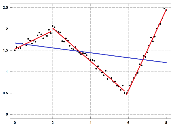
Figure 1: An example of linear regression (in blue) and segmented linear regression (in red) for a given dataset (in black): the approximation with 3 line segments offers a significantly better accuracy than linear regression.
Segmented Linear Regression
Segmented linear regression (SLR) addresses this issue by offering piecewise linear approximation of a given dataset [2]. It splits the dataset into a list of subsets with adjacent ranges and then for each range finds linear regression, which normally has much better accuracy than one line regression for the whole dataset. It offers an approximation of the dataset by a sequence of line segments. In this context, segmented linear regression can be viewed as a decomposition of a given large dataset into a relatively small set of simple objects that provide compact but approximate representation of the given dataset within a specified accuracy.
Segmented linear regression provides quite robust approximation. This strength comes from the fact that linear regression does not impose constraints on ends of a line segment. For this reason, in segmented linear regression, two consecutive line segments normally do not have a common end point. This property is important for practical applications, since it enables us to analyse discontinuities in temporal data: sharp and sudden changes in the magnitude of a signal, switching between quasi-stable states. This method allows us to understand the dynamics of a system or an effect. For comparison, high degree polynomial regression provides a continuous approximation [3]. Its interpolation and extrapolation suffer from overfitting oscillations [4]. Polynomial regression is not a reliable predictor in applications mentioned earlier.
Despite the simple idea, segmented linear regression is not a trivial algorithm when it comes to its implementation. Unlike linear regression, the number of segments in an acceptable approximation is unknown. The specification of the number of segments is not a practical option, since a blind choice produces usually a result that badly represents a given dataset. Similarly, uniform splitting a given dataset into equal-sized subsets is not effective for achieving an optimal approximation result.
Instead of these options, we place the restriction of the allowed deviation and attempt to construct an approximation that guarantees the required accuracy with as few line segments as possible. The line segments detected by the algorithm reveal essential features of a given dataset.
The deviation at a specified x value is defined as the absolute difference between original and approximation y values. The accuracy of linear regression in a range and the approximation error are defined as the maximum of all of the values of the deviations in the range. The maximum allowed deviation (tolerance) is an important user interface parameter of the model. It controls the total number and lengths of segments in a computed segmented linear regression. If input value of this parameter is very large, there is no splitting of a given dataset. The result is just one line segment of linear regression. If input value is very small, then the result may have many short segments.
It is interesting to note that within this formulation, the problem of segmented linear regression is similar to the problem of polyline simplification. The solution to this problem provides the algorithm of Ramer, Douglas and Peucker [5]. Nevertheless, there are important reasons why polyline simplification is not the best choice for noisy data. This algorithm gives first priority to data points the most distant from already constructed approximation line segments. In the context of this algorithm, such data points are the most significant. The issue is that in the presence of noise, the significant points normally arise from high frequency fluctuations. The biggest damage is caused by outliers. For this reason, noise can have substantial effect on the accuracy of polyline simplification. In piecewise linear regression, each line segment is balanced against the effect of noise. The short term fluctuations are removed to show significant long term features and trends in original data.
Algorithms
Adaptive Subdivision
Here, we discuss two algorithms for segmented linear regression. In the attached code, the top level functions of these algorithms are SegmentedRegressionThorough()and SegmentedRegressionFast(). Both of them are based on adaptive subdivision, which we borrow from the solution to polyline simplification. Figure 2 shows the top-down dynamics of this method.

Figure 2: Illustration of an adaptive recursive subdivision for data stored in an array. The top array represents a given dataset. Each subdivision improves linear regression in two proper arrays at a lower level. The resulting subdivision arrays with required approximation accuracy are located at the deepest level. Note that the arrays are not equal-sized.
The pseudo-code of this subdivision method is given below:
StackRanges     stack_ranges ;
stack_ranges.push( range_top(0, n_values) ) ;

while ( !stack_ranges.empty() )
{
    range_top = stack_ranges.top() ;
    stack_ranges.pop() ;

    if ( CanSplitRange( range_top, idx_split, ... ) )
    {
        stack_ranges.push( range_left (range_top.idx_a, idx_split      ) ) ;
        stack_ranges.push( range_right(idx_split      , range_top.idx_b) ) ;
    }
    else
        ranges_result.push_back( range_top ) ;
}
The criterion of splitting a range, implemented in both algorithms (see the function CanSplitRangeThorough() and CanSplitRangeFast()), is based on the comparison of approximation errors against user provided tolerance. A range is added to the approximation result as soon as the specified accuracy has been achieved for each approximation value in the range. Otherwise, it is split into two new ranges, which are pushed onto stack for subsequent processing.
These two functions also implement the test for a small indivisible range. It is necessary to avoid confusion that can be caused by the subdivision of a dataset with two data elements only. The current version of the algorithms is not allowed to create a degenerate line segment that corresponds to one datum.
This method of subdivision belongs to the family of divide-and-conquer algorithms. It is fast and guarantees space efficiency of its result. Under the simplifying assumption that the cost of a single split operation is constant, the running time of the recursive subdivision is O(N) in the worst case and O(log M) on average, where N is the number of elements in a given dataset and M is the number of line segments in a resulting approximation. The cost of a split operation is specific to a particular algorithm. This effect on overall performance is discussed below.
The obvious question now is how to find the best split points for the recursive subdivision that we just discussed? It appears that there is more than one method to answer this key question. These methods are responsible for a bit different approximation results and for different performance of SLR algorithms. We start the discussion with the simple method, which is easier to understand than the second more advanced method.
Sequential Search for the Best Split
The simple method (see function CanSplitRangeThorough()) represents a sequential search for the best split point in a range of a given dataset. It involves the following computational steps: A currently selected data point provides us with two sub-ranges. For each sub-range, we compute several sums, parameters of linear regression and then the accuracy of the approximation as the maximum of absolute differences between original and approximation y values. The best split point is defined by the best approximation accuracy for both sub-ranges.
Figure 3: Segmented linear regression using sequential search for the best split point. The sample noisy data (in black) were obtained from daily stock prices. The lower accuracy approximation (in green) has 3 segments. The higher accuracy approximation (in red) has 13 segments.
This simple method (see Figure 3) delivers good approximation results in terms of compactness: a small number of line segments for a specified tolerance, but unfortunately it is too slow and not practical for processing large and huge datasets. The weakness of this algorithm is that linear cost of sequential search for the best split in a given range (see function CanSplitRangeThorough()) is multiplied by linear cost of the computation of linear regression in sub-ranges. Thus, the total running time of this algorithm is at least quadratic. In the worst case of linear performance of the recursive subdivision, this algorithm becomes cubic. This speed cannot be improved significantly by using tables of pre-computed sums. The bottleneck is the computation of approximation errors in a range, which takes linear time.
Search Using Simple Moving Average
The efficiency of an algorithm that builds segmented linear regression can be improved if we avoid the costly sequential search on each range discussed in the first algorithm. For this purpose, we need a fast method to detect a subset of data points that are the most suitable to split ranges in a given dataset.
In order to better understand the key idea of the faster algorithm, let us consider perfect input data without noise. Figure 4 shows the computation of simple moving average (SMA) [6] for sample data that have a number of well-defined line segments.
Figure 4: Simple moving average for sample data not affected by noise: original dataset in black, smoothed data in red, the absolute differences between original and smoothed data in blue. The vertical line illustrates the fact that positions of local maxima in the differences coincide with positions of local maxima and minima in the given data. The horizontal segment denotes smoothing window at a specific data point.
The important fact is that when SMA window is inside a range of original data with linear dependence y(x) each derived y value is equal to a matching original y value. In other words, the operation of smoothing based on SMA does not affect data points in ranges of linear dependence y(x) of original data. The deviations between original and derived y values become noticeable and increasing when smoothing window is moving into a range that covers more than one line segment. In a more general context, the smoothed curve is sensitive to all types of smooth and sharp non-linearities in original dataset, including "corners" and "jumps". The greater non-linearity, the greater the effect of the smoothing operation.
This feature of SMA suggests the following method to find ranges of linear dependence y(x) for the computation of local linear regression and break points between them. If we compute the array of absolute differences between original and smoothed values, then the required ranges of linear dependence in original data correspond to small (ideally zero) values of differences in this array. The break points between these approximation ranges are defined by local maxima in the array of differences.
In the algorithm implemented in the attached code (see function SegmentedRegressionFast()), we detect all local maxima in the array of absolute differences between original and smoothed data. The order of splitting approximation ranges (in function CanSplitRangeFast()) is determined by the magnitude of local maxima. For each new range of subdivision, we compute parameters and approximation error of linear regression. This processing stops as soon as a required accuracy has been achieved. It means that not all of the local maxima are normally used to build the approximation result.
When it comes to real life data affected by noise (see Figure 5), smoothing not only helps us to detect line segments in given data, but also allows us to measure the amount of noise in the data. The current version of this algorithm uses symmetric window. The length of the window provides control of the accuracy of linear approximation. In order to obtain smoothed data, we apply one smoothing operation to the whole input dataset. There is no need later to use smoothing in approximation ranges created by subdivision. This approach helps us to avoid issues associated with boundary conditions of SMA.
Figure 5: Segmented linear regression using simple moving average for the same data as in Figure 3. The lower accuracy approximation (in green) has 4 segments. The higher accuracy approximation (in red) has 13 segments.
It should be clear from this discussion that the choice of a smoothing method is important for this variant of piecewise linear regression. SMA is a low pass filter. Thus, it looks like other types of low pass filters are suitable for smoothing operation too. This is not impossible in theory, but it is unlikely that this is a good idea in practice. Compared to other types of low pass filters, SMA is one of the simplest and efficient. Its properties have been intensively studied. In particular, a well-known issue of SMA is that it can invert high frequency oscillations. For the algorithm discussed here, this will lead to a bit less accurate locating local maxima. This issue can be easily addressed with iterative SMA, which is known as Kolmogov-Zurbenko filter [7]. In addition, iterative SMA gives more control over the removal of high frequency fluctuations. Not only smoothing window length but also the number of iterations is available to reduce the amount of noise in derived data and to achieve the best possible approximation. Importantly, this iterative filter also preserves line segments of given data.
In terms of performance, the second SLR algorithm (function SegmentedRegressionFast()) has the important advantage over the first algorithm (function SegmentedRegressionThorough()). The costs of major algorithmic steps are not multiplied but added. The search for potential split points using local maxima in absolute differences between original and smoothed data is quite fast and is completed before the recursive subdivision. This search involves the computation of SMA, an array of differences and an array of local maxima. Since each of these computations takes linear time, this stage of algorithm also completes in linear time. The subsequent recursive subdivision operates on the given split points and only needs to compute parameters of local linear regression, which takes linear time. Thus, the average cost of this SLR algorithm is O(N log M) and the worst case cost is quadratic, where N is the number of elements in a given dataset and M is the number of line segments in resulting approximation. This performance is much better than that of the first algorithm. This is why the algorithm based on smoothing is the preferable choice for the analysis of large datasets.
The price of the improved performance is that the second algorithm may not find precise positions of split points that guarantee the highest accuracy of linear regression. This is often acceptable in real life applications, since the exact position of a local maximum in noisy data is a bit vague concept. This situation is similar to the analysis of smoothed data. An approximation is normally acceptable as soon as its smoothed curve is meaningful in the application context. A failure to find segmented linear regression when user tolerance is strict is not necessarily a bad feature of this algorithm. If there are two line segments in input data, the algorithm is not expect to detect ten approximation line segments. As an additional measure, the precision of finding best split points can be improved by using narrow sequential search in areas of local maxima only.
For large and huge datasets, the performance and accuracy can be controlled by combining two algorithms: First, we run fast algorithm based on SMA smoothing to detect significant split points. This result is used for initial partition of a given dataset to build the first order approximation. Then, we continue subdivision of the ranges of the first approximation with sequential search for split points that has better accuracy.
Concluding Remarks
It is interesting to note the implementation of both algorithms requires a small amount of code. The comments in the attached code are focused on the appropriate technical details. In this section, we discuss the other important aspects of the code and algorithms.
In order to focus on the main ideas of the algorithms, their implementation prioritizes readability of the code. For the same reason, we do not use the methods that address issues of numerical errors in computations, which involve floating-point numbers. This approach makes the code more portable to other languages. In this context, we note that class std::vector<T> represents a dynamic array. Also, the implementation is not optimized for the best performance. In particular, it does not use tables of pre-computed sums or advanced data structures.
As discussed before, the attached code does not support a user interface parameter for the minimal length of a range (the limit for indivisible range). The implementation of these general purpose algorithms applies the fundamental limit of 2 points for a line segment. Because of this, segmented linear regression can have many small line segments, which correspond to data subsets with small number of elements produced by subdivision process. This effect is usually caused by high frequency noise when user specified accuracy of approximation is too strict. Such a result most likely is not useful in practice. If this is the case, then it makes sense to introduce a larger limit for indivisible range to detect the failure at early stages of processing.
The algorithms discussed here assume that input data are equally spaced. It is possible to use these algorithms in special cases when deviations from this requirement are relatively small. However, in the general case, it is necessary to properly prepare input data. The issue of outliers is beyond the scope of this article, although it is very important in practice. The current implementation assumes that all input values are significant and none of them can be removed.
Segmented linear regression becomes ineffective when it contains a large number of small segments (loss of compactness) or its representation of data does not achieve a specified accuracy. Another complication is that segmented linear regression allows for more than one acceptable result. This fact makes its interpretation not as trivial as that of linear regression.
In practical applications, the naïve questions "what is noise?" and "what is signal?" quite often are hard to answer. However, without the knowledge of characteristics of noise, we cannot make reliable conclusions and meaningful predictions. The major challenge is to develop an adequate mathematical model for the data analysis. The models that work well are thoroughly tested against real life datasets.
Point of Interest
The performance measurements of algorithms are always of special interest, even though the running times may vary significantly from system to system. For the data shown in the tables below, the system tested was a desktop computer with AMD Ryzen 7 PRO 3700 processor, 16GB of RAM and Windows 10 Pro operating system. The code was generated in Visual Studio 2019 using console type of applications. The execution time was measured in milliseconds with Stopwatch in C# and with std::chrono::high_resolution_clock in C++. The first table shows the results for the SLR algorithm implemented in the function SegmentedRegressionThorough().
| N | 10,000 | 20,000 | 30,000 | 50,000 | 70,000 |
| C++ | 215 | 860 | 1,930 | 5,370 | 10,500 |
| C# | 560 | 2,240 | 5,030 | 13,900 | 27,500 |
The second table shows the results for the algorithm in the function SegmentedRegressionFast().
| N | 10,000 | 20,000 | 30,000 | 50,000 | 70,000 | 100,000 |
| C++ | 1.2 | 2.5 | 3.1 | 3.5 | 3.9 | 5.0 |
| C# | 6.3 | 9.9 | 13.3 | 12.7 | 13.3 | 15.5 |
The C++ and C# variants algorithms demonstrate similar dependence of the running time on the size of input dataset. The first algorithm based on sequential search is asymptotically consistent with the model of computational cost. The second algorithm using simple moving average is less trivial for the analysis, since its performance is more sensitive to the number of segments in a resulting approximation.
The comparison of the values of the running times of the same algorithms shows that C++ is about 3 times faster than C#. Nevertheless, it is more important to note that C# algorithm using simple moving average is significantly faster than C++ algorithm based on sequential search for the best split. The practical lesson from these measurements is that the choice of a right algorithm is more important than the choice of a programming language. C++ is not going to help us fix problems caused by brute force algorithms, whereas C# can deliver more than acceptable performance with a smart implementation.
References
- https://en.wikipedia.org/wiki/Linear_regression
- https://en.wikipedia.org/wiki/Segmented_regression
- https://en.wikipedia.org/wiki/Polynomial_regression
- https://en.wikipedia.org/wiki/Overfitting
- https://en.wikipedia.org/wiki/Ramer-Douglas-Peucker_algorithm
- https://en.wikipedia.org/wiki/Moving_average
- https://en.wikipedia.org/wiki/Kolmogorov-Zurbenko_filter
History
- 7th October, 2020: Initial version
- 20th October, 2020: Added source code in C#
- 2nd November, 2020: Added "Point of Interest" section
Vadim Stadnik has many years of experience of the development of innovative software products. He is the author of the book “Practical Algorithms on Large Datasets”, available on Amazon. His interests include computational mathematics, advanced data structures and algorithms, artificial intelligence and scientific programming.


 General
  News
News  Suggestion
  Question
  Bug
Bug  Answer
  Joke
Joke  Praise
  Rant
Rant  Admin
Admin 


 haha
haha
