Theory versus Practice?

• Download source code 3.6 MB
• Download sample of table function - 8.2 KB
• Download sample of numerical calculation - 5.5 KB
• Download Parametric Identification of Transfer Functions in the Frequency Domain - 6.9 KB
• Download Parametric Identification of Transfer Functions in the Frequency Domain (actual function) - 9 KB
• Download Artificial Earth Satellite sample - 1.5 MB

Useful links

• Universal engineering software homepage
• Weifen Luo homepage

1. Introduction

First stage of math education contains familiarization with numbers. Then unknown "x" was introduced. I thought: "Why do you need "x"? Does not application of numbers quite enough?" A lot of my friends had similar opinion. One my colleague told me similar story. Then he noticed that I have used notation f for real function of real argument. He said: "Your notation is not correct. You should use f(x) notation". I explained that f means actual function but f(x) is value of function where argument is equal to x (f(x) is also named potential function).  Indeed  usage of  f is next step of abstraction. A lot of people tell:"I do not theoretician I am practitioner" A lot of people told me that they are practitioners. But "practitioner" term as itself does not have meaning. So I asked  people: "Who is practitioner?" My public opinion poll yield following well known list of answers:

• I am an engineer, so I do not need object oriented paradigm. (This engineer had used ALGOL at 1995, he used a lot of labels instead "begin ... end" construction.
• I do not have no time for theoretical study.
• I prefer simplicity. (This man is not familiar with code reuse).
• High quality contradicts rapid development.

Any good IT specialist can himself/herself extend this list of antipatterns. My own opinion is: "Theory is useful for practice". So I placed "?" at this article title. All my articles contain a lot of theory. Main accent of this article is usefulness of theory. Following story proves that application of theory is time saving.

I was often condemned by my colleagues: “You are reading irrelevant books” One my colleague many years tried to find analytical solution of on engineering ordinary differential equation. I told him that existence of such solution is extraordinary event. I read the book I. Kaplansky, “Differential Algebra”, Hermann (1957). Roughly speaking this book explains the fact that existence of analytical solution is extraordinary event. The colleague answered me that the book is irrelevant. “We are not mathematicians but we are engineers” He did not find analytical solution. I am not sure that this solution would be useful because numerical solution takes part of one second. A lot of colleagues told me that they are very busy. So they do not read smart books. They told that I have a lot of time and so I read a lot of books. However I do not spend time for useless tasks. Maybe reading of smart books provides time-saving?

2. Background.

Rigorous math has laconism, definiteness and context dependence. Meaning of below notation

is presented in following table

N	Element	Type
1	f, g	Real function of real argument
2	a	Real number
3	v	Real vector which dimension is equal to n

My friend thought that "x" in "f(x)" is always real number. However "x" can be also a vector or a function. Following table represents different types of "x"

is presented in following table:

N	Type of argument	Expression	Meaning	Type of result
1	Real number	f(a)	Result of calculation of f if argument is equal to a	Real number
2	Real function of real argument	f(g)	Composition of functions f and g	Real function of real argument
1	Real vector which dimension is equal to n	f(v)	Componentwise calculation of f	Real vector which dimension is equal to n

Samples of applications of this theory is presented below.

3. Functions

3.1 Base interface

Talk about f and f(x) was happened at 1977. A lot of engineers thought that FORTRAN is the best language and at that time usefulness of theory was not evident for software development. Only object oriented paradigm provide good abstract expression of function. Following interface represents base interface for all one variable function:

 /// <summary>
/// Function of one variable
/// </summary>
public interface IOneVariableFunction : IObjectOperation
{
    /// <summary>
    /// Type of variable
    /// </summary>
    object VariableType
    {
        get;
    }
}

/// <summary>
/// Operation which returns an object
/// </summary>
public interface IObjectOperation
{

    /// <summary>
    /// Types of input parameters
    /// </summary>
    object[] InputTypes
    {
        get;
    }

    /// <summary>
    /// Calculates result of this operation
    /// </summary>
    /// <param name="arguments">Array of arguments</param>
    /// <returns>Operation result</returns>
    object this[object[] arguments]
    {
        get;
    }

    /// <summary>
    /// Return type
    /// </summary>
    object ReturnType
    {
        get;
    }

 }

Above interface is specification of IObjectOperation interface. The IObjectOperation very general interface which calculates object by set of arguments. The IOneVariableFunction is not always real function of real argument. The ReturnType and VariableType properties are types of function return and argument respectively.

3.2 Examples

3.2.1 Explicit formula

A set functions can be represented by explicit formula. Samples of explicit expressions are presented below:

These expressions represent the same function. However arguments of the functions are different. Moreover types of arguments p and t can be different.

3.2.2 Table

A lot of functions used in science and engineering are defined by experiment. These functions are tabulated. Example of tabulated function is presented below:

Following picture represents sample of application of tabulated function:

The Chart element is a table. Columns of this table are X (abscissa) and Y (ordinate). It have following outputs:

N	Parameter	Symbol	Type
1	Array of X values	X	double[dimension]
2	Array of Y values	Y	double[dimension]
3	Minimal element among X values	X_1	double
4	Minimal element among Y values	Y_1	double
5	Maximal element among X values	X_2	double
6	Maximal element among Y values	Y_2	double
7	Function f defined by table	Function	double f(double)

Following picture represents user interface of these parameters:

Follownig picture presents demo application of tabulated functions:

Properties of objects F, G and H are presented below

The F has single formula (Formula 1). The formula has single variable f. Otherwise the f variable is linked to Double f(Double) Function of Graph object. The G object has three variables and two output formulae.

N	Variable name	Type	Comment
1	f	Double f(Double)	Formula_1 of F
2	g	Double f(Double)	Function from Chart
3	t	Double	Time variable

N	Formula	Type	Comment
1	Formula_1	Double	Real value of function which depends on time variable
2	Formula_2	Double f(Double)	Composition of functions f and g

And at last H object has following variables and output formulae

<><>< />

N	Variable name	Type	Comment
1	x	Double	Formula_1 of G = Value of Chart function where argument equals to time
2	f	Double f(Double)	Formula_2 of G = Composition of Chart function and Formula_1 from F = Composition of Chart function with ifsels
3	t	Double	Time variable

N	Formula	Type	Comment
1	Formula_1	Double	Value of x = Value of Chart function where argument equals to time
2	Formula_2	Double	f(t) value, where f is composition of Chart function with itself, t is time

Following picture represents Formula_1 and Formula_1 of G.

Red and Blue curve are charts of Chart function and composition of Chart function with itself respectively. Note that this software assumes that X limits of table value of function equals to zero.

• Download this sample - 8.2 KB

3.2.3 Numerical calculation

There are a lot of math functions which do not have explicit expression. A lot of differential equations do not have explicit solutions. For example second order linear differential equation y''+xy = 0 (x is argument, '' means second total derivative) does not have explicit solution. The I. Kaplansky, “Differential Algebra”, Hermann (1957) book contains prove of above fact. However numerical calculation yield these functions. Here numerical solution of y''+xy = 0 is considered. This differential equation is equivalent to following system of first order differential equations:

y' = z;

z' = -xy.

where z = y'. We consider following modification of above system:

Greek delta means Dirac delta function, k and a are real constants. This modified system also does not have explicit solution but presence of delta function makes equations more interesting. Following picture represents solution of above system.

The Differential equation object has following properties:

Where variable a is Formula_1 of Input which is represented below

.

Following chart represents solution of differential equation system:

Red and blue curve represents y and z respectively. Jump of z is caused by presence of Dirac delta function as well as jump of y derivative. So numerical solution yield necessary function. However this function is rather f(x) than f. It is potential function, i.e. calculation for concrete value of argument. But a lot of tasks require actual f, i.e. function as global. For example composition of functions requires function as global. Application of following Accumulator component yield actual (global) f.

This component has following variables:

The Accumulator is very similar to Transport Delay of Simulink. Accumulator transfers potenial functions y(t), z(t) of Differential equation to actual ones, i.e. y and z respectively. These actual functions are numerically calculated on [0,1] interval. Step of calculation is equal to 0.01, number of steps is equal to 100. These actual functions can be composed. The Composition yield this composition. Properties of this component are presented below:

Variables of Composition are presented below

N	Variable name	Type	Comment
1	f	Double f(Double)	Differential_equation_y of Accumulator = y of Differential equation as actual function
2	g	Double f(Double)	Differential_equation_z of Accumulator = z of Differential equation as actual function

Output of Composition is function composition f(g) or y(x) because f and g of Composition are respectively actual y and z of Differential equation. Composition result is presented below:

• Download this sample

4. Practical Applications

Above samples are rather artificial then practical. Here I would like to prove usefulness of theory for practice.

4.1 Parametric Identification of Transfer Functions in the Frequency Domain

Here is a survey of Parametric Identification of Transfer Functions in the Frequency Domain. We would like identify parameters of following third order transfer function:

Assume that frequency response is defined by experiment. Following picture represents idea of identification is presented at following pictures.

We would like yield such values of constants k, T₁, T₂, T₃ that theoretical dependence of frequency response approximate experimental values. Experimental values are red crosses of above charts. Blue curves theoretically calculated frequency responses. Identification yield good approximation of experimental data. Theoretical dependencies of frequency response and phase response of above transfer function are presented below:

tan^-1 and phase response are expressed in degrees. So we would like approximate experimental data by above formula of frequency response. Following picture contains solution of this task

The Graph element contains following table of frequency response which yield experiment.

X and Y columns of this table correspond to frequency and frequency responce. The Formula component contains following regression formula:

Above formula is explicit expression of frequency response. Argument p of this formula is a vector (array) of Graph X coordinates. So argument of function is not real number but real vector. Constants of above formula correspond to parameters of transfer function by following way:

N	Constant of formula	Parameter of transfer function
1	k	k
2	a	T1
3	b	T2
4	c	T3

So above formula represents theoretical frequency response. The Processor component yield such values of k, T₁, T₂, T₁ (or k, a, b, c of Formula) that experimentally defined values of frequency response are approximated by theoretically calculated values. Properties of Processor component are presented below:

Number 0 correspond to both Formula_1 of Formula and Y of Graph. It means that experimentally defined values of frequency response is approximated by theoretical ones. All marked by -1 expressions are not taken into account in regression process. However Formula component has other formulae:

First formula is frequency response. But argument of this formula is time variable t. Second one is phase response. Application of these formulae is indication of frequency response:

• Download this sample - 6.9 KB 

Theoretical function f of frequency response is used twice. First of all it is used as f(p) where is vector. Also it is used as f(t) where t is (nonconstant) real number. Application of 2 formulae for single function is not a good idea. Following picture represents application of single function.

The Formula object calculates f(t), where t is time variable. Then Accumulator makes actual f from f(t). And at last F(X) object calculates application of this function to X - coordinates of Graph object. Properties of F(X) are presented below

• Download this sample - 9 KB

4.2 Artificial Earth satellite

Here following tasks are considered

• Determination of motion parameters;
• Generation of text document;
• Visualization;
• Audio support.

All these tasks use motion parameters as time functions in different context. Orbit determination uses vector values, visualization uses functions of time variable. However single set of parameters are being used for all this tasks. Roughly speaking actual f instead potential f(x) is used.

4.2.1 Motion model

Motion model of spacecraft is already described here. But I have copied text for easy reading.

The motion model of an artificial satellite is a system of ordinary differential equations that describe the motion in a Greenwich reference frame:

where are the coordinates and components of velocity respectively, is angular velocity of Earth, and are components of the summary external acceleration. The current model contains gravitational force and the aerodynamic one. These accelerations can be defined by the following formulae:

The following table contains meaning of these parameters:

Component of ordinary differential equations is used for above equations. This component does not have a rich system of symbols and uses lower case variables only. However this component supports rich system of comments which is presented below:

These comments can contain mappings between variables and physical parameters. Independent variables of equations (x, y, z, u, v, w) are checked in right part. Mapping between these variables and

The component represents differential equations in the following way:

Besides independent variables equations contain additional parameters. The following table contains mapping of these parameters:

Some of these parameters are constants. Other parameters should be exported. Constants are checked and exported parameters are not checked below:

Exported parameters concern with gravity and atmosphere models. These models are contained in external libraries. The following picture contains components of motion model.

The Motion equations component is considered above component of ordinary differential equations. These equations have feedback. Right parts of equations depend on gravitational forces. Otherwise gravitational forces depend on coordinates of the satellite. The Vector component is used as feedback of Motion equations.

This picture has the following meaning. Variables x, y, z, u, v, w of Vector component are assigned to x, y, z, u, v, w variables of Motion equations. Input and output parameters of Vector are presented below:

Components Gravity, Atmosphere are objects obtained from external libraries which calculate Gravity of Earth and Earth's atmosphere respectively. Both these objects implement IObjectTransformer interface. The G-transformation and A-transformation objects are helper objects which are used for application of Gravity, Atmosphere objects respectively. Properties of G-transformation are presented below:

The above picture has the following meaning. The G-transformation is connected to Gravity object. This object corresponds to exported Gravity class (code of Gravity class is above this text). The Gravity class implements IObjectTransformer interface. Input parameters of Gravity are coordinates which are labeled by "x", "y", "z" labels. So above comboboxes are labeled by x", "y", "z labels. The above picture means that parameters x", "y", "z" are assigned to Formula_1, Formula_2, Formula_3 of Vector component. Otherwise Formula_1, Formula_2, Formula_3 of Vector are assigned to x, y, z of Motion equations. However Motion equations component uses parameters of G-transformation:

This picture means that parameters a, b, c of a, of Motion equations are assigned to parameters Gx, Gy, Gz of G-transformation. So of Earth's

Gravity

function is exported to G-transformation. The Earth's atmosphere is exported in a similar way.

4.2.2 Orbit determination

The following picture illustrates the problem of determination of the orbit.

We have an artificial Earth's satellite. There are a set of ground stations which perform measurements. So we have measurements of distance and relative velocity between stations and the satellite. Processing of these measurements provides determination of orbit.

4.2.2.1 Input Data

Input data contains measurements of distances and relative velocities. Special components are used for this purpose. These components are presented below:

Ordinates of Distance component are measured distances and ordinates of Velocity one are measured relative velocities. Abscises of these components are indifferent. Other input data are represented below:

The full list of input parameters is represented in the following table:

	Component name	Comment
1	Distance	Array of distance measurements
2	Velocity	Array of velocity measurements
3	Distance Time	Array of times of distance measurements
4	Velocity Time	Array of times of velocity measurements
5	Distance X	Array of X - coordinates of ground station which correspond to distance measurements
6	Distance Y	Array of Y - coordinates of ground station which correspond to distance measurements
7	Distance Z	Array of Z - coordinates of ground station which correspond to distance measurements
8	Velocity X	Array of X - coordinates of ground station which correspond to velocity measurements
9	Velocity Y	Array of Y - coordinates of ground station which correspond to velocity measurements
10	Velocity Z	Array of Z - coordinates of ground station which correspond to velocity measurements
11	Distance Sigma	Array of standard deviations of distance measurements
12	Velocity Sigma	Array of standard deviations of velocity measurements

Let us comment on this table. We have two arrays of measurements. First array d₁, d₂, ... contains measurements of distance. Second one V₁, V₂ ... contains measurements of velocity. First two rows of the above table correspond to these two arrays. Measurements d₁, d₂, ... are performed in different times. Third row of above table corresponds to array of times of these measurements. Similarly 4 - th row corresponds to array of times of V₁, V₂ ... measurements. A set of ground stations is used for measurements. Suppose that d_i is obtained by ground station which has coordinates X_i, Y_i, Z_i. The 5, 6, 7 th rows of table correspond to X_i, Y_i, Z_i arrays. Similarly 8 - 10 rows correspond to coordinates of ground stations and V_i measurements. Note that the different measurements have no equal accuracy. The General linear method requires to use different weights for such measurements. A new component was developed for this purpose. It enables us to create weighted selections. In case of orbit determination, measurements have different variances. So we have weighted least squares situation. So variances of measurements are needed. Rows 11 and 12 contain arrays variances of d_i and V_i respectively. Components Distance Selection and Velocity Selection are "weighted selections" which contain measurements and their variances. Properties of Distance Selection are presented below:

This picture has the following meaning:

• Array of measurements is contained in ordinates of Distance component.
• Array of variances is contained in ordinates of Distance Sigma component.

The Velocity Selection component is constructed in a similar way. I've used the graph component for the storage of the selection. It has been done since the user would be able to try this example without a database. Really, this scenario should use the connection to the database graph .

4.2.2.2 Nonlinear Regression

Nonlinear regression in statistics is the problem of fitting a model.

to multidimensional x,y data, where f is a nonlinear function of x, with regression parameter θ.

Nonlinear regression operates with selections. This software implements two methods of manipulation with selections. The first method loads selection iteratively, i.e., step by step. The second one loads selection at once.

The architecture of nonlinear regression software that uses iterative regression is presented in the following scheme:

Let us describe the components of this scheme. The iterator provides data-in selections x and y. The y is the Left part of fitting the equations. The Transformation corresponds to the nonlinear function f, and generates the Left part of the fitting model. The Processor coordinates all the actions and corrects the Regression parameters.

The architecture of the software with loading selection at once is presented in the following scheme:

The processor compares Calculated parameters with Selection, calculates residuals, and then corrects Regression parameters. In these two schemas, the Iterator, Selection, and others are not concrete components. They are components that implement interfaces of Iterator, Selection etc. For example, a Camera component may implement the Selection interface. Here, I'll consider examples in brief. A more profound description is available in the documentation of this project. Second scheme is used for determination of orbits.

4.2.2.3 Ingredients

The above picture contains general ingredients of nonlinear regression. Let us consider ingredients related to orbit determination of orbits. The Selection is already considered in 6.1. Regression parameters are initial values of coordinates and components of velocity of the satellite. These parameters are contained in Motion equations component. These parameters are presented in the following picture:

As it is already noted, parameters x, y, x, u, v, w are coordinates and components of velocity. Top part of above picture contains values of these parameters before orbit determination. Bottom one contains values after orbit determination. These parameters are being changed during orbit determination. Transformation stage contains the following steps:

• Calculation of trajectory of satellite
• Calculation of time shifts
• Calculation of distances and velocities

The Accumulator component performs calculation of trajectory parameters as actual functions. Let us explain what is the actual function. There are two points of definitions of function. According to potential point function f(t) is calculation of f by known argument t. Actual point means that function f is single (actual) object. Actual function can be obtained from potential by calculation of values of f(t) at different values of t. The Motion equations component performs potential calculation of motion parameters and Accumulator object transforms these potential functions to actual ones. Properties of Accumulator are presented below:

According to these properties, Accumulator calculates f(t₀), f(t₁), f(t₂), ... where t₀ = 1770457504 (Start), t_i+1 - t_i = 10 (Step). Number of values of argument is equal to 2500 (Step count). So Accumulator stores f(t₀), f(t₁), f(t₂) and for any t₀ < t < t₂₅₀₀. Then f(t) is obtained by interpolation by polynom of third degree. It should be noted that measurements of distances and velocities are not instant since speed of light is finite. Ground station sends signal at t₁ time, then satellite sends reflected signal at t₂ time and then ground station receives signal at t₃ time. The time of measurement is t₃. However measurement of distance is not distance between satellite and station at t₃. It is equal (d₁ - d₂) / 2 where d₁ is distance between station at t₁ time and satellite at t₂ time and similarly d₂ is distance between station at t₃ time and satellite at t₂ time. The Difference and Time + Shift components enable us take into account this circumstance. Properties of Difference component are presented in the following picture:

Output of this component is used by Time + Shift. Properties of Time + Shift are presented below:

This component calculates arrays of times of reflection of signals by the satellites. Component Delta is helper. It has the following properties:

The Measurements component calculates measurements of distance and velocity. This component has the following properties:

This parameters are compared with selections. The Processor component performs such computation or (using another term) regression. Regression formula is presented below:

Processor component reflects this formula. Properties of this component are presented below:

Left part of above window corresponds to x of regression formula. In considered case components of x are coordinates and components of velocity. The following table contains components of vector x.

	Physical parameter	Identifier
1	X	Motion Equations/Motion Equations.x
2	Y	Motion Equations/Motion Equations.y
3	Z	Motion Equations/Motion Equations.z
4	Vx	Motion Equations/Motion Equations.u
5	Vy	Motion Equations/Motion Equations.v
6	Vz	Motion Equations/Motion Equations.w

Middle part of above window contains f(x) of regression formula. The f(x) vector contains two subvectors Formula_1 and Formula_2 which belong to Measurements components. These subvectors are calculated values of distances and velocities. Right part of above window corresponds to y of regression formula. Vector y contains two selections which correspond to distance and velocity measurements respectively. Click to Iterate button initiate step of nonlinear regression.

4.2.2.4 Resume

Orbit determination requires motion parameters as actual functions. Moreover shifted by time delay functions are required. However motion equations do not have explicit solution. So Accumulator component is used. Roughly speaking it transforms potential f(x) function to actual f one.

4.2.3 Orbit determination container

Above tasts are already described in my article. Here extended task is described. Orbit determination task is aggregated for more easy further development. Aggregation result is presented below:

Extended task is presented at following picture:

It contains also video, audio and document generation.

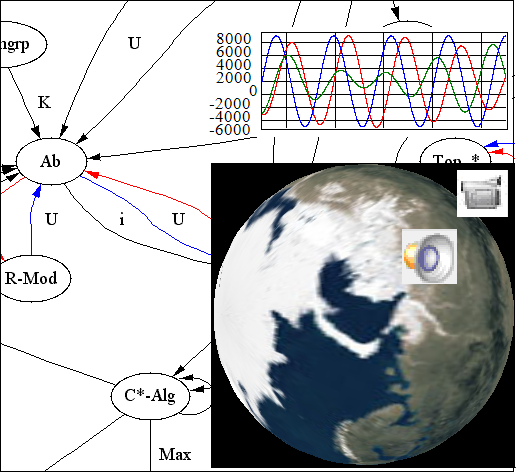
4.2.4 Video

Video task is rather "f(t)" than "f" where t is time variable. Following components are meant for video support:

 

The Camera component is virtual WPF Perspective Camera. It has following properties:

The Globe is 3D model of Globe. It contains XAML 3D model and texture. Globe and Camera are virtually installed on Base frame and Camera Frame respectively. Both Base frame and Camera Frame are virtual 3D Cartesian coordinate system These systems are meant for motion simulation of Camera with respect to Globe. Base frame is Greenwich reference frame. Other frames are constructed by following way:

This picture has following meaning. Motion of Frame 1, Frame 2, Camera Frame regarded as relative motion with respect to Base frame, Frame 1, Frame 2. Let x, y, z be coordinates of the satellite than Frame 1 has nonzero linear shift (x, y,z) with respect to Base frame. Also this frame is rotated by longitude around Z axis. Frame 2 is not shifted with respect to Frame 1. However it is rotated by latitude angle around Y - axis. Camera Frame has zero shift and following transformation matrix with respect to Frame 2

Visual image of these frames is presented below:

Where are latitude and longitude of the satellite respectively. Axes of Frame 1 are parallel to axes of X'Y'Z', both frames are red at above picture. However center of Frame 1 coincides with center of mass of the satellite. Axes of Frame 2 are parallel to axes of X''Y''Z'', both frames are blue at above picture and of Frame 2 also coincides with center of mass of the satellite. Components Angles and Quaternions are meant for orientation calculations. Properties of Angles are presented below:

Variables x, y, z are just coordinates x, y, z of the satellite. Formula_1, Formula_2 are exactly longitude and latitude of the satellite respectively. Rotation of Frame 1 and Frame 1 can be expressed by following quaternions respectively:

Quaternions component calculates necessary data for above quaternions. Properties of Quaternions component are presented below:

Following pictures and tables represent properties of Frame 1 and Frame 2

.

Properties of Frame 1

N	Parameter name	Frame parameter	Imported parameter	Comment
1	X	X - relative shift of frame	Orbit determination/Motion equations/Motion equations.x	X coordinate of the satellite
2	Y	Y - relative shift of frame	Orbit determination/Motion equations/Motion equations.y	Y coordinate of the satellite
3	Z	Z - relative shift of frame	Orbit determination/Motion equations/Motion equations.z	Z coordinate of the satellite
4	Q0	Real component of quaternion	Quaternions.Formula_1	cos(longitude/2)
5	Q1	i - component of quaternion	Quaternions.Formula_5	0
6	Q2	j - component of quaternion	Quaternions.Formula_5	0
7	Q3	k - component of quaternion	Quaternions.Formula_2	sin(longitude/2)

Properties of Frame 2

N	Parameter name	Frame parameter	Imported parameter	Comment
1	X	X - relative shift of frame	Quaternions.Formula_5	0
2	Y	Y - relative shift of frame	Quaternions.Formula_5	0
3	Z	Z - relative shift of frame	Quaternions.Formula_5	0
4	Q0	Real component of quaternion	Quaternions.Formula_1	cos(latitude/2)
5	Q1	i - component of quaternion	Quaternions.Formula_5	0
6	Q2	j - component of quaternion	Quaternions.Formula_5	sin(latitude/2)
7	Q3	k - component of quaternion	Quaternions.Formula_2	0

Camera frame is meant for Camera optical axis orientation in the direction to center of Globe.

4.2.5 Audio

Let us consider following audio support which blows sounds when satellite intersects Equator.

Following sounds are included in audio support:

• Blowing of "Up" word if satellite is moved from South hemisphere to North one;
• Blowing of "Down" word if satellite is moved from North hemisphere to South one.

This task is also rather "f(t)" than "f" where t is time variable. Following picture represents components of this sample

The Sound Recursive is element which performs following reqursive calclulations:

y_n=z_n;

x_n=y_n-1;

where z_n is z - coordinate of satellite at n^th step of calculation. Since z > 0 at North hemisphere and z < 0 at South we have following condition of Equator intersection.

N	Condition	Meaning
1	zn-1 < 0) AND (zn > 0)	The satellite has intersected Equator from South hemisphere to North one
2	zn-1 > 0) AND (zn < 0)	The satellite has intersected Equator from North hemisphere to South one

The Sound formula component yields formulae of these conditions:

Sound component is meant for sound blowing according following table:

N	Condition parameter	Meaning	Sound file
1	Sound formula.Formula_1 = true	Satellite intersects equator plane from South to North	up.wav
2	Sound formula.Formula_2 = true	Satellite intersects equator plane from North to South	down.wav

4.2.6 Generation of document

In this sample actual function f is used. However this function has another argument. This argument is Z- coordinate of the satellite.

Besides calculation, any software needs generation of documents. Facilities generation of documents are exhibited on forecast problem. Forecast document contains parameters of satellite motion in times of equator intersections. The following picture explains the forecast problem:

Satellite moves along its orbit. Parameters of motion correspond to the time when it moves from South to North and intersects equator. Satellite intersects equator when its Z - coordinate is equal to 0. If we have coordinates and time as function of Z, then we can see necessary parameters are values of these functions where Z = 0. The following picture represents a solution of this task.

The Delay component has FunctionAccumulator type. This type is very similar to Transport delay of Simulink. However

FunctionAccumulator

is more advanced. Properties of Delay are presented below:

The Delay component is connected to Data to data one. It stores latest output values of Data. The Step count = 4 means that Delay stores 4 last values of each output parameters. The Formula_4 of data is Z coordinate of satellite. So all parameters of Delay are considered as functions of Z. Let us consider all components of forecast. The Satellite component is a container which contains Motion equations of the satellite. The Data component is connected to Motion equations and adds time parameters to motion parameters. Properties of Data are presented below:

.

The Recursive component is similar to Memory component of Simulink. This component calculates time delay of Z coordinate. Properties of the Recursive element are presented below:

The Condition element is used for determination of time of equator intersection. Properties of Condition are presented below:

Meaning of parameters of this component is contained in comments:

And at last, Output component contains calculation of forecast parameters. It has the following formulae:

The 86 400 number is number of seconds in a day. The time function converts double variable to DateTime. The b is condition of equator intersection. Input parameters are motion parameters as functions of Z. Full list of parameters is contained in the following comments:

And at last, Chart component has the following properties:

These properties have the following meaning. Output is performed when condition variable is true. In this case, condition is Formula_1 of Condition object. It is condition of equator intersection. Output parameters are Formula_1 - Formula_7 of Output object. Labels X, Y, Z, Vx, Vy, Vz are labels which are reflected in XML document. The XML document is presented below:

<Root>
  <Parameters>
    <Parameter Name="T" Value="Monday, June 28, 1999 11:17:05 PM.457" />
    <Parameter Name="X" Value="-6595.47050815637" />
    <Parameter Name="Y" Value="-2472.05799683873" />
    <Parameter Name="Z" Value="0" />
    <Parameter Name="Vx" Value="-0.541295154046453" />
    <Parameter Name="Vy" Value="1.46945520971716" />
    <Parameter Name="Vz" Value="7.45051367374592" />
  </Parameters>
  <Parameters>
    <Parameter Name="T" Value="Tuesday, June 29, 1999 12:55:08 AM.068" />
    <Parameter Name="X" Value="-7026.76544757067" />
    <Parameter Name="Y" Value="487.053173194772" />
    <Parameter Name="Z" Value="0" />
    <Parameter Name="Vx" Value="0.117122882887633" />
    <Parameter Name="Vy" Value="1.56173832654579" />
    <Parameter Name="Vz" Value="7.45055871464937" />
  </Parameters>
 <Root>

The first parameter has DateTime type and the other ones have

double

type. The XML document reflects this circumstance. The XSLT (Extensible Stylesheet Language Transformations) is used for generation of documents. The following code contains XSLT file.

<xsl:stylesheet version="1.0" xmlns:xsl=http://www.w3.org/1999/XSL/Transform 
    xmlns:msxsl="urn:schemas-microsoft-com:xslt"
    xmlns:user="urn:my-scripts">
  <xsl:template match="/">
    <html>
      <body>
        <p>
          <h1>Forecast</h1>
        </p>
        <xsl:apply-templates />
      </body>
    </html>
  </xsl:template>
  <xsl:template match="Parameters">
    <p></p>
    <p>
      <table border="1">
        <xsl:apply-templates />
      </table>
    </p>
  </xsl:template>
  <xsl:template match="Parameter">
    <xsl:apply-templates />
    <tr>
      <td>
        <xsl:value-of select="@Name" />
      </td>
      <td>
        <xsl:value-of select="@Value" />
      </td>
    </tr>
  </xsl:template>
</xsl:stylesheet>

This XSLT code provides the following HTML document.

T	Monday, June 28, 1999 11:17:05 PM.457
X	-6595.47050815637
Y	-2472.05799683873
Z	0
Vx	-0.541295154046453
Vy	1.46945520971716
Vz	7.45051367374592
T	Tuesday, June 29, 1999 12:55:08 AM.068
X	-7026.76544757067
Y	487.053173194772
Z	0
Vx	0.117122882887633
Vy	1.56173832654579
Vz	7.45055871464937

4.2.7 Short instruction

4.2.7.1 Unpack following archive

• Download files - 1.5 MB

4.2.7.2 Installation of audio files

Installation of audio files includes following steps.
Step 1. Copy SOUNDS directory to any directory.

Step 2. Setting directory of unpacked files by following way

4.2.7.3 Installation of containes

Copy Containers directory to directory of

Aviation.exe

file;

4.2.7.4 Start animation

Start

Aviation.exe

. Open

Orbit.cfa

file. Click following Animation button

Points of Interest

My chief told me: "Do not read smart books. If you continue your reading then you shall have a lot of ill-wishers." Chief was quite right. Really a had a lot of ill-wishers. However I continued reading of smart books.