Impulse noises detection and cancelation in music records

Download INDC.zip

Introduction

When listening to archival music records we often meet (or more precisely hear) the problem of impulse noises occurrence – so called ‘crackles’. It is getting worse when listening to vinyl records or cassette tapes.

There are many algorithms whose task is to remove such distortions – some are suitable for hardware implementation, some of them can be used only in offline implementations.

This article is to present adoption of identification method Exponentially Weighted Least Squares (EWLS) and next step error prediction analysis.

Despite the fact that this algorithm will be used to detect and cancel noise in recorded music, it can successfully be used to cancel impulse noise from any set of even multidimensional signals.

Acoustic signals

Acoustic signals which are present in our real world are time-continuous signals, and in this form are recorded on analog media such as vinyl records or cassettes.

Recording on the more modern digital data media (CDs, hard drives, Flash memory) requires digitization of the analog signal - sampling and quantization.

Sound frequencies heard by the human ear are in the range of about 20 kHz. According to Nyquist - Shannon theorem the sampling frequency should be at least twice of highest frequency peak in signal spectrum in order to avoid the effect of aliasing. In the processing of music we used set sampling frequency of 44.1 kHz.

In the article it will be assumed that processed signal is digital and was sampled correctly according to Nyquist – Shannon theorem.

Signal estimation

Digital acoustic signal can be consider as discrete time function f(t), where t = 0, 1, … represents normalized time. Let assume that next function values (signal samples) can be represented by autoregressive model (AR):

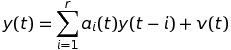
where  represents signal sample value in moment ,  represents time shift operator, represents rank of AR model, represents ith model parameter,  represents white noise.

Let us assume vectors:

and

Using them we are able to reorder autoregressive model equation:

If we will assume that vector  represents real (unknown to us) parameters of  signal, then we can assume that there is a vector  which is estimation of vector .

Recursive identification algorithms calculate prediction of next signal value  according to data (values) collected till this step:

Recursive identification algorithm

Due to equation above, if want to calculate signal value prediction for the next step we need to designate vector , as vector  is given as an outcome of previous operations.

To calculate  we will use Exponentially Weighed Least Squares algorithm. EWLS algorithm, as every in the least squares algorithms family, calculates model parameters by minimizing cost function on least squares – in EWLS it gives exponentially less weight to previous error values.

To reduce the impact of older values to the current calculation we need to assume a so called forgetting factor . The forgetting factor takes value from 0 to 1, wherein if  then EWLS algorithm’s memory is shorter.

The recursive EWLS is given with equation:

where  is an error function – the difference between true signal value in  moment and estimated signal value in  moment:

and  is a gain vector , described as:

where matrix  can be calculated with equation:

Interference detection

Impulse noises in two dimensional signal can be seen as samples with amplitude much higher than neighboring samples (Fig.1).

Fig.1. Impulse noise example in acoustic signal

To detect such a samples we will use algorithm based error function prediction, defined as

Let us declare two additional parameters, the first one is prediction error local variance:

the second one is standard deviation of prediction error:

Noise detection refers to verify the value of . Naturally, higher value of error function in  moment indicates that signal value in this moment is disturbed.

Obviously, the condition given above is strongly fuzzy – what does it mean ‘higher value of error function’?

To complete this condition we assume that suspicious samples of acoustic signal induce error function values above scaled standard deviation of this function:

where  is scaling coefficient which is responsible for algorithm sensitivity and need to be defined as algorithm input data. Note that too high  value may cause missing disturbed samples, whereas too low value may cause classifying ‘clean’ samples as disturbed ones.

Denote by  binary function with possible values 0 (if tth sample is ‘clean’) and 1 (if tth value is disturbed). Then:

Error prediction local variance can be calculated using:

with initial condition .

Reconstruction of distrubed samples

Sample marked as disturbed is to  be deleted and replaced with reconstructed one. For this purpose we will apply linear interpolation using neighboring ‘clean’ samples.

Another issue to be consider is the maximum number of next samples that can be disturbed. Due to this different  parameter value should be places in equation below

where indicates position of sample under reconstruction in the step.

Simulation

Initial parameter were taken in algorithm simulation:

A 20 second length music record was processed with algorithm, results can be seen at Fig. 2 and 3.

Fig.2. Simulation results. Upper plot presents original (disturbed) signal, lower plot presents this signal after detecting and canceling noises

Fig.3. Zoom of dataset from Fig. 2

Use of code

Implementation of this algorithm in Matlab environment is quite easy, as a lot of predefined functions can support us.

Use of code is by calling function:

impulse_noise_elimination(file_1, file_2, model_order, n, lambda, p, save_ar)

where:

%Function Impulse Noise Elimination input parametres:
% * file_1 is a name of input track, ex. 'music.wav';
% * file_2 is a name of output track, ex. 'music_mod.wav';
% * model_order is a choosen number of estimated model parameters; can be
%   choosen from range: 1 <= model_order <= 25; mostly the best choice is
%   model_order = 4;
% * n is a scaling coefficient of local variance in detecting algorithm;
%   its value decides of the level of impulse noise samples; mostly n = 3
%   is the best choice, but n is from range 2 <= n <= 20;
% * lambda is a memory coefficient in EW - LS algorithm; its value
%   dependends on track dynamic; lambda is from the range: 
%   0.001 (low dynamic) <= lambda <= 0.999 (high dynamic);
% * p is a scaling coefficient of P matrix (eye matrix rank model_order)
%   starting value; p is from range 10^3 <= p <= 10^6;
% * save_ar = 0 or 1; 0 if model parametres should not be saved, 1 if model
%   parameters should be saved.

Milestones of this function are shown below.

Input data check

[track fs tmp] = wavread(file_1); %orginal track (wav file)

round(model_order);
round(n);

if model_order > 25
    model_order = 25;
elseif model_order < 1
    model_order = 1;
end

if n > 20
    n = 20;
elseif n < 2
    n = 1;
end

if lambda > 1
    lambda = 0.999;
elseif lambda < 0
    lambda = 0.001;
end

if p < 1000
    p = 1000;
elseif p > 1000000
    p = 1000000;
end

if save_ar ~= 1
    save_ar = 0;
elseif save_ar == 1
    model_vector = zeros(max(size(track)), model_order);
end

Main loop steps

Initial parameters:

%Starting parametres of EW - LS algorithm:
org_track = track;
model = zeros(model_order, 1);
K = 0;
P = p * eye(model_order);
variance = 0;

Loop definition:

for t = (model_order + 1) : (max(size(track)) - 4)

% All operations

end

As it can be seen, loop start condition is

(model_order + 1)

wheras the end condition is 

(max(size(track)) - 4)

as we need to collect at least model rank samples number to start identification and our implemention considers that next four samples can be distrubed.

To get another signal value and calculate prediction error we do:

signal = track(t-1 : -1 : t-model_order);
prediction_error = track(t) - model' * signal;

When previous sample was 'clean', variance can be calculated:

variance = lambda*variance + (1 - lambda)*(prediction_error)^2;

Otherwise variance calculation does not change. To initiate we use:

variance = prediction_error^2;

The simplest (non-optimal) way to check next four samples (when first one is disturbed) is by using if condition:

if abs(prediction_error) > n * sqrt(variance) %detecting test
    
    noise_samples = 1;
    signal_1 = track(t : -1 : t-model_order+1);
    prediction_error_1 = track(t+1) - model' * signal_1;

    if abs(prediction_error_1) > n * sqrt(variance)
        
        noise_samples = 2;
        signal_2 = track(t+1 : -1 : t-model_order+2);
        prediction_error_2 = track(t+2) - model' * signal_2;
        
        if abs(prediction_error_2) > n * sqrt(variance)
                        
            noise_samples = 3;
            signal_3 = track(t+2 : -1 : t-model_order+3);
            prediction_error_3 = track(t+3) - model' * signal_3;
            
            if abs(prediction_error_3) > n * sqrt(variance)
                
                noise_samples = 4;
                
            end
        end
    end

else
    noise_samples = 0;
    variance = lambda*variance + (1 - lambda)*(prediction_error)^2;
end

After that we can try to reconstruct disturbed samples:

if noise_samples ~= 0
    for i = 0 : noise_samples - 1
        track(t + i) = track(t-1) + (-1 / (noise_samples + 1))*(track(t-1) - track(t + noise_samples))*(i+1);
    end
    noise_samples = 0;
end

At the end we can update our estimator parameters

prediction_error = track(t) - model' * signal;
K = (P * signal) / (lambda + signal'*P*signal);
P = (1 / lambda)*(P - (P*signal*signal'*P)/(lambda + signal'*P*signal));
model = model + K * prediction_error;

and start all over again.

Conclusion

Presented recursive algorithm can be implemented in real-time applications. The delay produced by this algorithm is defined by the maximum number of next samples that can be disturbed.

Acoustic signals considered in this article by the nature are characterized by their high dynamic of amplitude changes. Due to this are signals types can successfully be processed with this algorithm (for example measurement data).

References

[1] Niedźwiecki M. Kłaput T. Fast recursive basis function estimators for identification of time-varying processes., IEEE Transactions on signal processing, vol. 50, no. 8, pp. 1925 - 1934. August, 2002.

[2] Söderström T. Stoica P. System identyfication. Prentice-Hall International, Hemel Hempstead, 1989.

[3] Zieliński Tomasz P. Cyfrowe przetwarzanie sygnałów. Wydawnictwa Komunikacji i Łączności, Warszawa, 2005.