Fluid Surface Identification
Liquids are fluids that have a free surface (that is, a surface whose shape is not defined by its container). This article—the 17th in the series—describes how to identify a fluid surface. You can use this information to render the surface or to help compute surface tension.
Part 1 in this series summarized fluid dynamics; part 2 surveyed fluid simulation techniques. Part 3 and part 4 presented a vortex-particle fluid simulation with two-way fluid-body interactions that run in real time. Part 5 profiled and optimized that simulation code. Part 6 described a differential method for computing velocity from vorticity, and part 7 showed how to integrate a fluid simulation into a typical particle system. Part 8 explained how a vortex-based fluid simulation handles variable density in a fluid; part 9 described how to approximate buoyant and gravitational forces on a body immersed in a fluid with varying density. Part 10 described how density varies with temperature, how heat transfers throughout a fluid, and how heat transfers between bodies and fluid. Part 11 added combustion, a chemical reaction that generates heat. Part 12 explained how improper sampling caused unwanted jerky motion and described how to mitigate it. Part 13 added convex polytopes and lift-like forces. Part 14 modified those polytopes to represent rudimentary containers. Part 15 described a rudimentary Smoothed Particle Hydrodynamics (SPH) fluid simulation used to model a fluid in a container. Part 16 explored one way to apply SPH formulae to the Vortex Particle Method.
Indicator Function
The fluid simulation keeps track of the distribution of density throughout the domain. If you quantized the density distribution to have only two values (0 and 1), it would indicate where the fluid is and is not. Such a function is called an indicator function, as shown in Figure 1. The surface of a fluid lies on the boundary between where the indicator is 0 and 1. If you identify those transitions, you would identify the fluid surface.
Indicator function along a ray, passing through an object
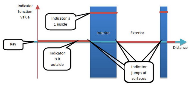
Figure 1. Indicator function
One problem: An indicator function does not lend itself well to tracking surfaces as they move. Say that you use some well-defined, noise-free density distribution to identify the fluid surface. Afterwards, you could advect the surface itself, just as you advect passive tracers or vortons. A problem arises, however: How would you represent the surface? You could represent it as a collection of polygons, then advect the vertices as passive tracer particles, but doing so would lead to problems. For example, what if the simulation started with two blobs of fluid that later merged (Figure 2)? Or a single blob that divided? Such events have topological changes—changes in the continuity of the fluid surface. Tracking the surface in that way would be highly problematic.

Figure 2. Topological changes to fluid surfaces. Two blobs merging or one blob dividing.
Although tracking surface motion using an indicator function creates more problems than it solves, it is still useful to identify surfaces in this way, at least initially. Later, I provide a better solution for tracking surface motion, but for the moment let’s see how to use the indicator function to identify a surface.
Finding Surfaces Using the Indicator Function
The fact that you’re tracking a fluid surface implies that the fluid has at least two components—for example, air and water. In an ideal incompressible fluid, each component would have uniform density within that component. Let’s call the density inside the water ρinside and the density outside water ρoutside.
Note: Remember from Part 3 that the simulation uses vortons to carry density but the fluid also has density even where it lacks vortons—that is, the fluid has an ambient density in the absence of vortons. Furthermore, because of numerical inaccuracies, vortons can converge and diverge, so the density is not exactly uniform throughout either component. This is a minor detail, but keep it in mind, because it affects the algorithm slightly.
Identifying the surface is easier on a uniform grid, so start by transferring density to a grid. Part 3 described just such an algorithm, and this new code reuses the same density grid.
The basic idea is straightforward, but its implementation becomes complicated in three dimensions. So, first consider one dimension (1D), where the concepts are easier to understand, then work toward higher dimensions case by case. Each case has a notion of a cell, which is a neighborhood of grid points. We want to find surface crossings inside each cell.
Each grid point has an associated density value. The algorithm finds where density transitions between an inside value and an outside value. In 1D, a cell is just the line segment between two adjacent grid points, and the surface is a single point along that segment. Figure 3 provides an example.
Figure 3. Finding transitions between outside and inside values. P and Q are samples with outside values of density. A is a sample with the value Z < A < M. B is a sample with the value Z < B < M. S values are estimates of where the indicator function transitions between outside and inside. M values are samples with the maximum value of the density. x are locations of samples; h are spacings between samples. The surface lies at each z, points where the indicator function transitions to an outside value. Assume that the value of x between Q and A, where the surface occurs, is linearly proportional to A/M. If I(xi)| < I(xi+1), then z = xi + hi(1 - A/M). If I(xi) > I(xi+1), then z = xi + hi(A/M).
This idea lets you identify surfaces, but how would you represent that information as data? In other words, given that you can compute where a surface crossing occurs within a cell, how should you store that information? The next section explains one way to do it.
Signed Distance Function
A signed distance function (SDF) describes, for each point in a domain, the distance to the nearest surface. Figure 4 shows an example.
SDF along a ray, passing through an object
Figure 4. Signed distance function
For each grid point around a cell that contains a surface crossing, you could store how far that point is to the surface crossing. In other words, you can encode, at each grid point adjacent to a surface crossing, the SDF to the nearest surface. In 1D, you could use density as an indicator to find surface crossings and encode their distances to each neighboring grid point.
The idea becomes more complicated in two dimensions (2D) and the implementation even more so. In 2D, a cell is a quadrilateral. Instead of considering each line segment between pairs of grid points (as in 1D), in 2D you must consider quadruples of grid points. You still start by finding surface crossings between adjacent grid points, as in the 1D case. Each cell can have zero to four surface crossings on its boundary, and each configuration leads to zero, one, or two line segments that terminate at surface crossings—that is, the surface inside a 2D cell is either one line segment or two line segments. Figure 5 provides an example.
Figure 5. Finding signed distance in 2D. The signed distance for each grid point depends on the shortest distance to a line segment. In some cases, that happens to be the distance to the nearest surface crossing point on the cell boundary. In other cases, that turns out to be the distance to the line passing through two surface crossings on cell boundaries.
In three dimensions, you must consider box-shaped cells instead of quadrilaterals, and the situation becomes even more complex. Each box has 12 edges, each of which might have a surface crossing. Each surface crossing is a vertex of a polygon that coincides with the surface. Furthermore, unlike in 1D or 2D, even when you know all the surface crossings, you cannot tell the topology of the polygons without looking at neighboring cells.
All of these problems have solutions, but for the sake of brevity, leave the details aside for the moment. Given a cell of density values (and neighboring cells), you can find the surfaces within that cell.
Given some algorithm that tells us where surfaces lie inside a cell, how should you represent that information? You could generate polygon meshes, as described above, but that leads to problems when you track how that surface moves. If you use signed distance instead, it makes tracking easier. (Later, I’ll explain how and why.)
An algorithm like the following would assign signed distance values to each grid point adjacent to a surface crossing:
- Given:
- A uniform grid of density values;
- The density outside the fluid of interest, ρoutside; and
- The density inside the fluid of interest, ρinside.
- Do:
- Compute ρdenominator = ρinside - ρoutside;
- Create a uniform grid of floating-point SDF values that has the same geometry as the density grid;
- Initialize the SDF uniform grid to have all FLT_MAX values;
- Create a uniform grid of Boolean SDF-pinned values that has the same geometry as the density grid;
- Initialize the SDF-pinned values to false; and
- For each grid point…
- For each adjacent grid point in {x, y, z}…
- Find its density, ρadjacent.
- If the current and adjacent grid points lie on opposite sides of a surface…
- Find the distance to the surface.
- Conditionally update the SDF for the grid points.
See ComputeImmediateSDFFromDensity_Nearest in the accompanying code for details.
The SDF-pinned grid simply indicates for which grid points the SDF has a value. That probably seems redundant, but it will come in handy later. Ignore it for the moment.
Running this algorithm gives you a uniform grid of SDF values but only immediately adjacent to surface crossings. The rest of the domain effectively has unassigned values.
When tracking surface motion, it is useful to know the SDF values farther away from the surface. The next section explains how to fill in remaining SDF values, given some established SDF values (the pinned values).
The Eikonal Equation
You want to populate a grid of SDF values, given that only some of them have been assigned. This problem turns out to be the same as solving a partial differential equation constrained by boundary conditions. The boundary conditions are, of course, that the SDF is known at certain (pinned) locations (which came from the algorithm above). The differential equation of interest expresses that the difference in SDF, u, between any two points is equal in magnitude to the distance those two points:
This is a special case of the Eikonal equation. The word Eikonal derives from the same Greek root as icon, meaning image because it describes the propagation of light rays. The idea behind solving the Eikonal equation is to cast rays along surface normal and assign SDF values as you march along each ray. That procedure would work, but it’s not the most efficient solution.
You can also solve this equation by visiting each point in the grid and propagating SDF values from neighboring grid points (see Figure 6).
Figure 6. Propagating SDF values between neighboring grid points. The heavy black line depicts the surface. Arrows depict the propagation of SDF values away from the surface into the rest of the domain. Note that the SDF values in this picture are quantized to line segments. The actual SDF would be smoother—for example, it would have rounded corners if the grid had infinite resolution.
Naïvely, the pseudo-code for this approach would look simple:
- For each grid point:
- Solve the finite difference using the Eikonal equation.
This algorithm resembles the Gauss-Seidel algorithm part 6 used to solve the Poisson equation. But this algorithm has some problems when applied to the Eikonal equation. As when solving the Poisson equation, solving the Eikonal equation at each grid point requires already having a solution at all neighboring grid points used by the finite difference scheme. But unlike when solving the Poisson equation, solutions to the Eikonal equation propagate in only one direction: downwind. Information propagates downwind from the source, where the source is a region with a solved, pinned value. For the Eikonal equation, the finite difference stencil uses only upwind values—that is, values that come from the direction opposite that of the information propagation.
Remember, the grid starts with some grid points where the SDF is known (and pinned). Imagine, for example, that initial known values reside within the interior of the domain. If a solver algorithm started at the zeroth (e.g., upper-left) grid point and progressed in the direction of increasing index values (e.g., downward and rightward), then it would have no upwind neighbors, so there would be no way to assign that grid point a value. If, instead, a solver started at the last grid point and progressed in the direction of decreasing index values, then the last grid point would have no upwind neighbors, so there would be no way to assign a value for that grid point. The solution, then, entails making multiple passes through the grid, one with positive increments and one with negative increments, for each axis in {x,y,z}. This yields a total of eight passes through the grid:
- {-,-,-}
- {+,-,-}
- {-,+,-}
- {+,+,-}
- {-,-,+}
- {+,-,+}
- {-,+,+}
- {+,+,+}
The routine ComputeRemainingSDFFromImmediateSDF_Nearest_Block in the accompanying code implements this algorithm, but first read the next section to understand how that routine is used.
Using Wavefronts to Parallelize the Eikonal Equation Solver
How would you parallelize the Eikonal solver? Because it resembles the Gauss-Seidel Poisson solver, you might be tempted to take the same approach part 6 describes: Slice the domain and issue threads to solve each slice. As with the Poisson solver, the solution at each grid point depends on the solution at adjacent grid points, so a red-black ordering might come to mind. But the Eikonal equation solution propagates strictly from sources outward, so the solution requires respecting that propagation.
Think of the SDF as a substance carried by a breeze that flows away from sources (surfaces). Before you can compute the SDF at a grid point, you must first compute the SDF at its predecessors—those grid points that are upwind. To parallelize this algorithm, the solver must have some way to add jobs to a queue, where those jobs correspond to the grid points whose upwind predecessors already have solutions. You add a job to solve the equation in a region only after you have solved all of the inputs for that region.
Intel® Threading Building Blocks (Intel® TBB) provides parallel_do, which helps with such problems. The magic of parallel_do is feeders. The worker routine is given a chunk of work to do and a feeder. The feeder lets the worker add chunks of work. So, as the worker completes some chunk of work, it can determine whether that finished chunk unblocks some future chunk and, if so, feed that chunk to Intel TBB. Later, Intel TBB will schedule that new chunk; parallel_do stops running when its job queue is empty.
You could make chunks of work equal to grid points, but the parallel_do machinery costs some overhead. It’s therefore better to aggregate multiple grid points into larger chunks. Hypothetically, the smallest chunk would be a grid point, and the largest would be the entire domain. Smaller chunks lead to finer granularity and better parallelism but have higher overhead. Larger chunks have coarser granularity and worse parallelism but lower overhead. To choose the optimal chunk size, profile the problem across various chunk sizes to see which size leads to the fastest run time.
Blocks
The code accompanying this article uses a Block structure to represent a chunk of work. A block represents a region within a uniform grid. Each block has an index triple: its x, y, and z indices.
struct Block
{
int mBlockIndices[ 3 ] ;
Block has helper routines to find the beginning and ending block of a domain that is subdivided, given a block size.
int BeginR( size_t axis , const int voxelsPerBlock[ 3 ] , const int numGridPoints[ 3 ] , const int inc[ 3 ] ) const
{
const int shift = ( inc[ axis ] > 0 ) ? 0 : 1 ;
const int unconstrained = ( mBlockIndices[ axis ] + shift ) * voxelsPerBlock[ axis ] ;
return Min2( unconstrained , numGridPoints[ axis ] - 1 ) ;
}
int EndR( size_t axis , const int voxelsPerBlock[ 3 ] , const int numGridPoints[ 3 ] , const int inc[ 3 ] ) const
{
const int begin = BeginR( axis , voxelsPerBlock , numGridPoints , inc ) ;
if( inc[ axis ] > 0 )
{
const int unconstrained = begin + voxelsPerBlock[ axis ] ;
return Min2( unconstrained , numGridPoints[ axis ] ) ;
}
else
{
const int unconstrained = begin - voxelsPerBlock[ axis ] ;
return Max2( unconstrained , -1 ) ;
}
}
} ;
Worker Functor
In the customary style of Intel TBB, create a functor to perform the work:
class ComputeRemainingSDFFromImmediateSDF_Nearest_TBB
{
UniformGrid< float > & mSignedDistanceGrid ; const UniformGrid< int > & mSdfPinnedGrid ; int mInc[ 3 ] ; int mVoxelsPerBlock[ 3 ] ; tbb::atomic< int > * mPendingPredecessorCount ; mutable tbb::atomic< bool > mutexLock ;
The function-call operator describes the worker process:
void operator() ( const Block & block , tbb::parallel_do_feeder< Block > & feeder ) const
{
    SetFloatingPointControlWord( mMasterThreadFloatingPointControlWord ) ;
    SetMmxControlStatusRegister( mMasterThreadMmxControlStatusRegister ) ;
    ComputeRemainingSDFFromImmediateSDF_Nearest_Block( mSignedDistanceGrid , mSdfPinnedGrid , mVoxelsPerBlock , mInc , block ) ;
    int nextIndices[ 3 ] = { block.mBlockIndices[ 0 ] + mInc[ 0 ]
                           , block.mBlockIndices[ 1 ] + mInc[ 1 ]
                           , block.mBlockIndices[ 2 ] + mInc[ 2 ] } ;
    FeedBlockToLoop( feeder, nextIndices, 0,         nextIndices[ 0 ] , block.mBlockIndices[ 1 ] , block.mBlockIndices[ 2 ] ) ;
    FeedBlockToLoop( feeder, nextIndices, 1, block.mBlockIndices[ 0 ] ,         nextIndices[ 1 ] , block.mBlockIndices[ 2 ] ) ;
    FeedBlockToLoop( feeder, nextIndices, 2, block.mBlockIndices[ 0 ] , block.mBlockIndices[ 1 ] ,         nextIndices[ 2 ] ) ;
}
The helper routine FeedBlockToLoop feeds new work to the thread scheduler:
void FeedBlockToLoop( tbb::parallel_do_feeder< Block > & feeder , const int nextIndices[ 3 ] , const int axis
, int ix , int iy , int iz ) const
{
if( nextIndices[ axis ] != EndBlock( axis ) )
{
if( -- Predecessor( ix , iy , iz ) == 0 )
{
feeder.add( Block( ix , iy , iz ) ) ;
}
}
}
This routine does the magical part: It keeps track of how many pending predecessor blocks each block is waiting on. When that count reaches zero, FeedBlockToLoop feeds the block to the loop.
Note the use of an atomic integer to keep track of the number of pending predecessor blocks. It has to be atomic because multiple threads could try to decrement or read that value concurrently. Intel TBB provides atomic integers to make that easy. The Predecessor routine is just a convenience accessor for that atomic<int>:
tbb::atomic< int > & Predecessor( int ix , int iy , int iz ) const
{
    const size_t offset = ix + NumBlocks( 0 ) * ( iy + NumBlocks( 1 ) * iz ) ;
    ASSERT( mPendingPredecessorCount[ offset ] >= 0 ) ;
    return mPendingPredecessorCount[ offset ] ;
}
Before kicking off the work, you have to initialize the functor:
void Init( int incX , int incY , int incZ )
{
const int numBlocksX = NumBlocks( 0 ) ;
const int numBlocksY = NumBlocks( 1 ) ;
const int numBlocksZ = NumBlocks( 2 ) ;
const int numBlocks = numBlocksX * numBlocksY * numBlocksZ ;
mInc[ 0 ] = incX ;
mInc[ 1 ] = incY ;
mInc[ 2 ] = incZ ;
mPendingPredecessorCount = new tbb::atomic< int >[ numBlocks ] ;
int beginBlock[ 3 ];
BeginBlock( beginBlock ) ;
for( int iz = 0 ; iz < numBlocksZ ; ++ iz )
for( int iy = 0 ; iy < numBlocksY ; ++ iy )
for( int ix = 0 ; ix < numBlocksX ; ++ ix )
{
const size_t offset = ix + numBlocksX * ( iy + numBlocksY * iz ) ;
mPendingPredecessorCount[ offset ] = ( ix != beginBlock[0] ) + ( iy != beginBlock[1] ) + ( iz != beginBlock[2] ) ;
}
}
Init allocates and initializes the pending predecessor count array.
Note that the beginning block (the first block to process) depends on the direction of propagation . . .
void BeginBlock( int indices[ 3 ] ) const
{
    for( int axis = 0 ; axis < 3 ; ++ axis )
    {
        if( mInc[ axis ] > 0 )
        {
            indices[ axis ] = 0 ;
        }
        else
        {
            indices[ axis ] = NumBlocks( axis ) - 1 ;
        }
    }
}
. . . because of the reason cited above: To solve the Eikonal equation, the solver has to make multiple passes, one that can handle each octant of characteristic directions that the solution can propagate.
The Driver routine kicks off the job:
static void Driver( UniformGrid< float > & signedDistanceGrid , const UniformGrid< int > & sdfPinnedGrid )
{
static const int voxelsPerBlock[ 3 ] = { 8 , 8 , 8 } ;
ComputeRemainingSDFFromImmediateSDF_Nearest_TBB functor( signedDistanceGrid , sdfPinnedGrid , voxelsPerBlock ) ;
static const int numPasses = 8 ;
for( int pass = 0 ; pass < numPasses ; ++ pass )
{
if( 0 == ( pass & 1 ))
{
functor.Init( -1 , -1 , -1 ) ;
}
else
{
functor.Init( 1 , 1 , 1 ) ;
}
Block rootBlock ;
functor.BeginBlock( rootBlock.mBlockIndices ) ;
tbb::parallel_do( & rootBlock , & rootBlock + 1 , functor ) ;
}
}
Note that in this case, the parallel_do routine is given a single block to work on. That’s not much of a workload. All work except for that first block gets fed to Intel TBB through the worker itself.
The result is that the work propagates diagonally across the domain, following a wavefront, as Figure 7 depicts. Hence, this pattern of parallelization is called a wavefront pattern.
Figure 7. Wavefront pattern
Summary
This article showed how to identify fluid surfaces using an indicator function to initialize signed distance values, how to populate the remainder of a domain with signed distance values by solving the Eikonal equation, and how to use Intel TBB to parallelize the Eikonal solver, using the wavefront parallel programming pattern.
Future Articles
The particle rendering used in the accompanying code is poor for liquids. It would be better to render only the liquid surface. This article described how to identify a surface. A later article will describe how to extract a polygon mesh from that to let you render the surface. You could use surface information to model surface tension, also a topic for a future article.
Particle methods, including SPH and vortex, rely on spatial partitioning to accelerate neighbor searches. The uniform grid used in this series is simplistic and not the most efficient, and populating it takes more time than it should. It would be worthwhile to investigate various spatial partition algorithms to see which runs fastest, especially with the benefit of multiple threads. Future articles will investigate these issues.
Further Reading
Related Articles
Fluid Simulation for Video Games (part 1)
Fluid Simulation for Video Games (part 2)
Fluid Simulation for Video Games (part 3)
Fluid Simulation for Video Games (part 4)
Fluid Simulation for Video Games (part 5)
Fluid Simulation for Video Games (part 6)
Fluid Simulation for Video Games (part 7)
Fluid Simulation for Video Games (part 8)
Fluid Simulation for Video Games (part 9)
Fluid Simulation for Video Games (part 10)
Fluid Simulation for Video Games (part 11)
Fluid Simulation for Video Games (part 12)
Fluid Simulation for Video Games (part 13)
Fluid Simulation for Video Games (part 14)
Fluid Simulation for Video Games (part 15)
Fluid Simulation for Video Games (part 16)
Any software source code reprinted in this document is furnished under a software license and may only be used or copied in accordance with the terms of that license.
Intel and the Intel logo are trademarks of Intel Corporation in the U.S. and/or other countries.
Copyright © 2013 Intel Corporation. All rights reserved.
*Other names and brands may be claimed as the property of others.
Dr. Michael J. Gourlay works as a principal lead software development engineer on new platforms including those meant for interactive entertainment. He previously worked at Electronic Arts (EA Sports) as the software architect for the Football Sports Business Unit, as a senior lead engineer on Madden NFL, on character physics and the procedural animation system used by EA on Mixed Martial Arts, and as a lead programmer on NASCAR. He wrote the visual effects system used in EA games worldwide and patented algorithms for interactive, high-bandwidth online applications. He also developed curricula for and taught at the University of Central Florida, Florida Interactive Entertainment Academy, an interdisciplinary graduate program that teaches programmers, producers, and artists how to make video games and training simulations. Prior to joining EA, he performed scientific research using computational fluid dynamics and the world’s largest massively parallel supercomputers. His previous research also includes nonlinear dynamics in quantum mechanical systems and atomic, molecular, and optical physics. Michael received his degrees in physics and philosophy from Georgia Tech and the University of Colorado at Boulder.


