The main objective of this article is to introduce you to the basics of Keras framework and use with other known libraries to make a quick experiment and take the first conclusions.
Introduction
Supervised Deep Learning is widely used for machine learning, i.e., computer vision systems. In this article, we will see some key notes for using supervised deep learning using the Keras framework.
Keras is a high level framework for machine learning that we can code in Python and it can be run in the most known machine learning frameworks like TensorFlow, CNTK, or Theano. It was developed in order to make the experimentation process easy and quick.
Background
This article doesn't give you an introduction to deep learning. You are supposed to know the basics of deep learning and a little of Python coding. The main objective of this article is to introduce you to the basics of Keras framework and use with other known libraries to make a quick experiment and take the first conclusions.
Using the Code
In this first article, we will train a simple neural net and, for the next articles, we will see some known deep learning architectures and make some comparisons.
All the experiments are done for educational purposes and the train process will be very quick and the results won't be perfect.
First Step: Load Libraries
First, we will load the libraries we need: numpy, TensorFlow (in this experiment, we will run Keras with this framework), Keras, Scikit Learn, Pandas... and more.
import numpy as np
from scipy import misc
from PIL import Image
import glob
import matplotlib.pyplot as plt
import scipy.misc
from matplotlib.pyplot import imshow
%matplotlib inline
from IPython.display import SVG
import cv2
import seaborn as sn
import pandas as pd
import pickle
from keras import layers
from keras.layers import Flatten, Input, Add, Dense, Activation,
                  ZeroPadding2D, BatchNormalization, Flatten,
                  Conv2D, AveragePooling2D,
                  MaxPooling2D, GlobalMaxPooling2D, Dropout
from keras.models import Sequential, Model, load_model
from keras.preprocessing import image
from keras.preprocessing.image import load_img
from keras.preprocessing.image import img_to_array
from keras.applications.imagenet_utils import decode_predictions
from keras.utils import layer_utils, np_utils
from keras.utils.data_utils import get_file
from keras.applications.imagenet_utils import preprocess_input
from keras.utils.vis_utils import model_to_dot
from keras.utils import plot_model
from keras.initializers import glorot_uniform
from keras import losses
import keras.backend as K
from keras.callbacks import ModelCheckpoint
from sklearn.metrics import confusion_matrix, classification_report
import tensorflow as tf
Set Up Datasets
For this exercise, we will use the CIFAR-100 dataset. This dataset has been used for a long time. It has 600 images per class with a total of 100 classes. It has 500 images for training and 100 images for validation per each class. Every one of the 100 classes are grouped in 20 superclasses. Each image has one "fine" label (the main class) and a "coarse" label (it superclass).
Keras framework has the module for direct download:
from keras.datasets import cifar100

(x_train_original, y_train_original),
(x_test_original, y_test_original) = cifar100.load_data(label_mode='fine')
Actually, we have downloaded the train and test datasets. x_train_original and x_test_original have the train and test images respectively, whereas y_train_original and y_test_original have the labels.
Let's see the y_train_original:
array([[19], [29], [ 0], ..., [ 3], [ 7], [73]])
As you can see, it is an array where each number corresponds to a label. Then, the first thing we have to do is convert these arrays to the one-hot-encoding version (see Wikipedia).
y_train = np_utils.to_categorical(y_train_original, 100)

y_test = np_utils.to_categorical(y_test_original, 100)
OK, now, let's see the train dataset (x_train_original):
array([[[255, 255, 255],
[255, 255, 255],
[255, 255, 255],
...,
[195, 205, 193],
[212, 224, 204],
[182, 194, 167]],

[[255, 255, 255],
[254, 254, 254],
[254, 254, 254],
...,
[170, 176, 150],
[161, 168, 130],
[146, 154, 113]],

[[255, 255, 255],
[254, 254, 254],
[255, 255, 255],
...,
[189, 199, 169],
[166, 178, 130],
[121, 133, 87]],

...,

[[148, 185, 79],
[142, 182, 57],
[140, 179, 60],
...,
[ 30, 17, 1],
[ 65, 62, 15],
[ 76, 77, 20]],

[[122, 157, 66],
[120, 155, 58],
[126, 160, 71],
...,
[ 22, 16, 3],
[ 97, 112, 56],
[141, 161, 87]],

...and more...

], dtype=uint8)
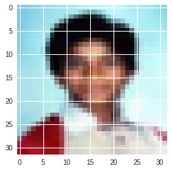
This dataset represents the 3 channels of 256 RGB pixels. Want to see it?
imgplot = plt.imshow(x_train_original[3])

plt.show()
Next, we have to normalize the images. That is, divide each element of the dataset by the total pixel number: 255. Once this is done, the array will have values between 0 and 1.
x_train = x_train_original/255

x_test = x_test_original/255
Setting Up the Training Environment
Before training, we have to set two parameters in Keras environment. First, we have to tell Keras where in the array are the channels. In an image array, channels can be in the last index or in the first. This is known channels first or channels last. In our exercise, we will set to channel last.
K.set_image_data_format('channels_last')
And the second thing is to tell Keras which phase it is. In our case, learning phase.
K.set_learning_phase(1)
Training a Simple Neural Net

We will train a simple neural net, so we have to code the method to return a simple neural net model.
def create_simple_nn():
  model = Sequential()
  model.add(Flatten(input_shape=(32, 32, 3), name="Input_layer"))
  model.add(Dense(1000, activation='relu', name="Hidden_layer_1"))
  model.add(Dense(500, activation='relu', name="Hidden_layer_2"))
  model.add(Dense(100, activation='softmax', name="Output_layer"))

  return model
Some keynotes from the code. The Flatten instruction converts the inputs (image matrix) in a one dimension array. Next, Dense instruction, adds a hidden layer to the model. The first hidden layer will have 1000 nodes, the second 500 and the third (output layer) 100. In the hidden layers, we will use the ReLu activation function and, for the output layer, the SoftMax function.
Once the model is defined, we compile it specifying optimization function, the loss function and the metrics we want to use. In all articles of this series, we will use exactly the same functions. We will use the Stochastic Gradient Descent optimization function, the Categorical Cross Entropy loss function and the accuracy and mse (Average of Cuadratic Errors) metrics. All of them are precoded in Keras.
snn_model = create_simple_nn()
snn_model.compile(loss='categorical_crossentropy', optimizer='sgd', metrics=['acc', 'mse'])
Once done, let's see the model summary.
snn_model.summary()
_________________________________________________________________
Layer (type) Output Shape Param
=================================================================
Input_layer (Flatten) (None, 3072) 0
_________________________________________________________________
Hidden_layer_1 (Dense) (None, 1000) 3073000
_________________________________________________________________
Hidden_layer_2 (Dense) (None, 500) 500500
_________________________________________________________________
Output_layer (Dense) (None, 100) 50100
=================================================================
Total params: 3,623,600
Trainable params: 3,623,600
Non-trainable params: 0
_________________________________________________________________
As we can see, despite being a simple neural network model, it has to train more than 3 million parameters. This will be the main reason for the existence of the Deep learning because if you want to train very complex networks, it would be necessary to train large amounts of parameters in this way.
Now, we just have to train. Do the following:
snn = snn_model.fit(x=x_train, y=y_train, batch_size=32,
      epochs=10, verbose=1, validation_data=(x_test, y_test), shuffle=True)
We tell Keras we want to use for training the train normalized image dataset and the one-hot-encoding train labelled array. We will use batches of 32 blocks (for reducing the use of memory) and we will take 10 epochs. For validation, we will use x_test and y_test. The training results will be assigned to the snn variable. From that, we will extract the training history for making comparisons between models.
Train on 50000 samples, validate on 10000 samples
Epoch 1/10
50000/50000 [==============================] - 16s 318us/step - loss: 4.1750 -
acc: 0.0740 - mean_squared_error: 0.0097 - val_loss: 3.9633 - val_acc: 0.1051 -
val_mean_squared_error: 0.0096
Epoch 2/10
50000/50000 [==============================] - 15s 301us/step - loss: 3.7919 -
acc: 0.1298 - mean_squared_error: 0.0095 - val_loss: 3.7409 - val_acc: 0.1427 -
val_mean_squared_error: 0.0094
Epoch 3/10
50000/50000 [==============================] - 15s 294us/step - loss: 3.6357 -
acc: 0.1579 - mean_squared_error: 0.0093 - val_loss: 3.6429 - val_acc: 0.1525 -
val_mean_squared_error: 0.0093
Epoch 4/10
50000/50000 [==============================] - 15s 301us/step - loss: 3.5300 -
acc: 0.1758 - mean_squared_error: 0.0092 - val_loss: 3.6055 - val_acc: 0.1626 -
val_mean_squared_error: 0.0093
Epoch 5/10
50000/50000 [==============================] - 15s 300us/step - loss: 3.4461 -
acc: 0.1904 - mean_squared_error: 0.0091 - val_loss: 3.5030 - val_acc: 0.1812 -
val_mean_squared_error: 0.0092
Epoch 6/10
50000/50000 [==============================] - 15s 301us/step - loss: 3.3714 -
acc: 0.2039 - mean_squared_error: 0.0090 - val_loss: 3.4600 - val_acc: 0.1912 -
val_mean_squared_error: 0.0091
Epoch 7/10
50000/50000 [==============================] - 15s 301us/step - loss: 3.3050 -
acc: 0.2153 - mean_squared_error: 0.0089 - val_loss: 3.4329 - val_acc: 0.1938 -
val_mean_squared_error: 0.0091
Epoch 8/10
50000/50000 [==============================] - 15s 300us/step - loss: 3.2464 -
acc: 0.2275 - mean_squared_error: 0.0089 - val_loss: 3.3965 - val_acc: 0.2013 -
val_mean_squared_error: 0.0090
Epoch 9/10
50000/50000 [==============================] - 15s 301us/step - loss: 3.1902 -
acc: 0.2361 - mean_squared_error: 0.0088 - val_loss: 3.3371 - val_acc: 0.2133 -
val_mean_squared_error: 0.0089
Epoch 10/10
50000/50000 [==============================] - 15s 299us/step - loss: 3.1354 -
acc: 0.2484 - mean_squared_error: 0.0087 - val_loss: 3.3233 - val_acc: 0.2154 -
val_mean_squared_error: 0.0089
Despite the fact that we have been evaluating the training during the training, we should use a new test dataset. I expose how to do it in Keras.
evaluation = snn_model.evaluate(x=x_test, y=y_test, batch_size=32, verbose=1)
evaluation

10000/10000 [==============================] - 1s 127us/step
[3.323309226989746, 0.2154, 0.008915210169553756]
Let's see the results metrics graphically (we will use the matplotlib library).
plt.figure(0)
plt.plot(snn.history['acc'],'r')
plt.plot(snn.history['val_acc'],'g')
plt.xticks(np.arange(0, 11, 2.0))
plt.rcParams['figure.figsize'] = (8, 6)
plt.xlabel("Num of Epochs")
plt.ylabel("Accuracy")
plt.title("Training Accuracy vs Validation Accuracy")
plt.legend(['train','validation'])

plt.figure(1)
plt.plot(snn.history['loss'],'r')
plt.plot(snn.history['val_loss'],'g')
plt.xticks(np.arange(0, 11, 2.0))
plt.rcParams['figure.figsize'] = (8, 6)
plt.xlabel("Num of Epochs")
plt.ylabel("Loss")
plt.title("Training Loss vs Validation Loss")
plt.legend(['train','validation'])

plt.show()
Well, at first, the model doesn't generalize well, If you see, there is an accuracy difference of 4%.
Confusion Matrix using SciKit Learn
Once we have trained our model, we want to see another metrics before taking any conclusion of the usability of the model we have been created. For this, we will create the confusion matrix and, from that, we well see the precision, recall y F1-score metrics (see wikipedia).
To create the confusion matrix, we need to make the predictions over the test set and then, we can create the confusion matrix and show that metrics. Each higher value of the array of predictions will be the real prediction. Really, the usual way is to take a bias value to discriminate if a prediction value can be positive.
snn_pred = snn_model.predict(x_test, batch_size=32, verbose=1)
snn_predicted = np.argmax(snn_pred, axis=1)
The Scikit Learn library has the methods to make the confusion matrix.
snn_cm = confusion_matrix(np.argmax(y_test, axis=1), snn_predicted)
snn_df_cm = pd.DataFrame(snn_cm, range(100), range(100))
plt.figure(figsize = (20,14))
sn.set(font_scale=1.4)
sn.heatmap(snn_df_cm, annot=True, annot_kws={"size": 12})
plt.show()
At last, show metrics:
snn_report = classification_report(np.argmax(y_test, axis=1), snn_predicted)
print(snn_report)

             precision    recall  f1-score   support

          0       0.47      0.32      0.38       100
          1       0.29      0.34      0.31       100
          2       0.24      0.12      0.16       100
          3       0.14      0.10      0.12       100
          4       0.06      0.02      0.03       100
          5       0.14      0.17      0.16       100
          6       0.19      0.13      0.15       100
          7       0.14      0.26      0.19       100
          8       0.22      0.18      0.20       100
          9       0.23      0.39      0.29       100
         10       0.29      0.02      0.04       100
         11       0.27      0.09      0.14       100
         12       0.34      0.23      0.28       100
         13       0.26      0.16      0.20       100
         14       0.19      0.13      0.15       100
         15       0.16      0.14      0.15       100
         16       0.28      0.19      0.23       100
         17       0.32      0.25      0.28       100
         18       0.18      0.26      0.21       100
         19       0.42      0.08      0.13       100
         20       0.35      0.45      0.40       100
         21       0.27      0.43      0.33       100
         22       0.27      0.18      0.22       100
         23       0.30      0.46      0.37       100
         24       0.49      0.31      0.38       100
         25       0.14      0.10      0.11       100
         26       0.17      0.11      0.13       100
         27       0.06      0.29      0.09       100
         28       0.32      0.37      0.34       100
         29       0.12      0.21      0.15       100
         30       0.50      0.13      0.21       100
         31       0.24      0.04      0.07       100
         32       0.29      0.19      0.23       100
         33       0.18      0.28      0.22       100
         34       0.17      0.03      0.05       100
         35       0.17      0.07      0.10       100
         36       0.21      0.19      0.20       100
         37       0.24      0.06      0.10       100
         38       0.17      0.06      0.09       100
         39       0.12      0.07      0.09       100
         40       0.26      0.23      0.24       100
         41       0.62      0.45      0.52       100
         42       0.10      0.05      0.07       100
         43       0.09      0.44      0.16       100
         44       0.10      0.12      0.11       100
         45       0.20      0.03      0.05       100
         46       0.22      0.19      0.20       100
         47       0.37      0.19      0.25       100
         48       0.14      0.48      0.22       100
         49       0.38      0.11      0.17       100
         50       0.14      0.05      0.07       100
         51       0.16      0.15      0.16       100
         52       0.43      0.60      0.50       100
         53       0.27      0.61      0.37       100
         54       0.48      0.26      0.34       100
         55       0.07      0.01      0.02       100
         56       0.45      0.13      0.20       100
         57       0.10      0.42      0.16       100
         58       0.35      0.17      0.23       100
         59       0.13      0.36      0.19       100
         60       0.40      0.65      0.50       100
         61       0.42      0.34      0.38       100
         62       0.25      0.49      0.33       100
         63       0.31      0.21      0.25       100
         64       0.14      0.03      0.05       100
         65       0.13      0.02      0.03       100
         66       0.00      0.00      0.00       100
         67       0.20      0.35      0.25       100
         68       0.24      0.66      0.35       100
         69       0.26      0.30      0.28       100
         70       0.37      0.22      0.28       100
         71       0.37      0.46      0.41       100
         72       0.11      0.01      0.02       100
         73       0.22      0.22      0.22       100
         74       0.09      0.06      0.07       100
         75       0.27      0.28      0.27       100
         76       0.29      0.38      0.33       100
         77       0.20      0.01      0.02       100
         78       0.19      0.03      0.05       100
         79       0.25      0.02      0.04       100
         80       0.14      0.02      0.04       100
         81       0.13      0.02      0.03       100
         82       0.59      0.50      0.54       100
         83       0.14      0.15      0.14       100
         84       0.18      0.06      0.09       100
         85       0.20      0.52      0.28       100
         86       0.31      0.23      0.26       100
         87       0.21      0.27      0.23       100
         88       0.07      0.02      0.03       100
         89       0.16      0.44      0.24       100
         90       0.20      0.03      0.05       100
         91       0.30      0.34      0.32       100
         92       0.20      0.10      0.13       100
         93       0.18      0.17      0.17       100
         94       0.46      0.25      0.32       100
         95       0.23      0.41      0.29       100
         96       0.24      0.17      0.20       100
         97       0.10      0.16      0.12       100
         98       0.09      0.13      0.11       100
         99       0.39      0.15      0.22       100

avg / total       0.24      0.22      0.20     10000
ROC Curve
The ROC curve is used by binary classifiers because it is a good tool to see the true positives rate versus false positives.
We will code the ROC curve for a multiclass classification. This code is from DloLogy, but you can go to the Scikit Learn documentation page.
from sklearn.datasets import make_classification
from sklearn.preprocessing import label_binarize
from scipy import interp
from itertools import cycle
n_classes = 100
from sklearn.metrics import roc_curve, auc
lw = 2
fpr = dict()
tpr = dict()
roc_auc = dict()
for i in range(n_classes):
fpr[i], tpr[i], _ = roc_curve(y_test[:, i], snn_pred[:, i])
roc_auc[i] = auc(fpr[i], tpr[i])
fpr["micro"], tpr["micro"], _ = roc_curve(y_test.ravel(), snn_pred.ravel())
roc_auc["micro"] = auc(fpr["micro"], tpr["micro"])
all_fpr = np.unique(np.concatenate([fpr[i] for i in range(n_classes)]))
mean_tpr = np.zeros_like(all_fpr)
for i in range(n_classes):
mean_tpr += interp(all_fpr, fpr[i], tpr[i])
mean_tpr /= n_classes
fpr["macro"] = all_fpr
tpr["macro"] = mean_tpr
roc_auc["macro"] = auc(fpr["macro"], tpr["macro"])
plt.figure(1)
plt.plot(fpr["micro"], tpr["micro"],
label='micro-average ROC curve (area = {0:0.2f})'
''.format(roc_auc["micro"]),
color='deeppink', linestyle=':', linewidth=4)
plt.plot(fpr["macro"], tpr["macro"],
label='macro-average ROC curve (area = {0:0.2f})'
''.format(roc_auc["macro"]),
color='navy', linestyle=':', linewidth=4)
colors = cycle(['aqua', 'darkorange', 'cornflowerblue'])
for i, color in zip(range(n_classes-97), colors):
plt.plot(fpr[i], tpr[i], color=color, lw=lw,
label='ROC curve of class {0} (area = {1:0.2f})'
''.format(i, roc_auc[i]))
plt.plot([0, 1], [0, 1], 'k--', lw=lw)
plt.xlim([0.0, 1.0])
plt.ylim([0.0, 1.05])
plt.xlabel('False Positive Rate')
plt.ylabel('True Positive Rate')
plt.title('Some extension of Receiver operating characteristic to multi-class')
plt.legend(loc="lower right")
plt.show()
plt.figure(2)
plt.xlim(0, 0.2)
plt.ylim(0.8, 1)
plt.plot(fpr["micro"], tpr["micro"],
label='micro-average ROC curve (area = {0:0.2f})'
''.format(roc_auc["micro"]),
color='deeppink', linestyle=':', linewidth=4)
plt.plot(fpr["macro"], tpr["macro"],
label='macro-average ROC curve (area = {0:0.2f})'
''.format(roc_auc["macro"]),
color='navy', linestyle=':', linewidth=4)
colors = cycle(['aqua', 'darkorange', 'cornflowerblue'])
for i, color in zip(range(3), colors):
plt.plot(fpr[i], tpr[i], color=color, lw=lw,
label='ROC curve of class {0} (area = {1:0.2f})'
''.format(i, roc_auc[i]))
plt.plot([0, 1], [0, 1], 'k--', lw=lw)
plt.xlabel('False Positive Rate')
plt.ylabel('True Positive Rate')
plt.title('Some extension of Receiver operating characteristic to multi-class')
plt.legend(loc="lower right")
plt.show()
Finally, we will save the train history data.
with open(path_base + '/simplenn_history.txt', 'wb') as file_pi:
pickle.dump(snn.history, file_pi)
Points of Interest
Despite training 10 epochs with this model is good enough, we see in the graphics of accuracy and loss that the model will not improve much better by taking more epochs. The ROC curve has a good true positive rate versus the false positive rate (means that when predict one class label, it have a low rate to be a false positive). Anyway, the rate is so much low for the accuracy, recall and precision.
In the next chapter, we will train the same dataset with a very simple convolutional neural network also using the same metrics, and loss and optimization functions. See you soon!
History
- 20th May, 2018: Initial version


 General
  News
News  Suggestion
  Question
  Bug
Bug  Answer
  Joke
Joke  Praise
  Rant
Rant  Admin
Admin 


