Recurrence plots in C#, extending WinRQA application

• Download sample data - 51.6 KB
• Download the source code for the WinRQA project - 1 MB

Introduction

WinRQA is a Windows application, written in C#, dedicated to the recurrence plots and recurrence analysis. In the first article about this application, I posted a first basic version of the application. In the present article, I post a new release with some useful tools. (If you prefer to read a spanish version, you can visit my blog).

The changes made in this release are the following:

• Now, you can read csv files with more than one time series (columns must be separated by a semicolon). This way, you can, by example, work with complete theoretical systems and compare them with simplified versions of them, built from a single time series from those in the whole system.
• The cross recurrence plots now can be rectangular, if the two system have different window size. This is the correct approach in this type of recurrence plots. Also, some minor inaccuracies have been corrected in the calculations of the recurrence quantification measures.
• I have added a tool to draw the changes of the linear autocorrelation of the series along with the changes in the delay. This can help us to select the correct value for the delay used in the recurrence plot.
• I have added also a tool similar to the former, but using the mutual information instead of linear correaltion. This can help to select the delay from a non linear point of view.
• Finally, I have added another graphical tool to help us to select the embedding dimension, using the correlation dimension as a reference.

Using the new features

Here is a image of the application with the new tool windows:

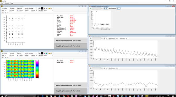
In the main recurrence plot window, there is now a third toolbar to access to the tools.

The AC button launches the autocorrelation tool, the MI button the mutual information tool, and the ED button is for the embedding dimension tool.

The autocorrelation tool window is as follows:

With the  button, the autocorrelation of the series will be calculated, from a distance (delay) of 1 to the maximum distance selected in the Max Distance text box.

With the  buttons you can select the range of the series values used to calculate the autocorrelation. You can select independently start at the beginning of the entire time series or at the beginning of the window used to build the recurrence plot. The same is valid for the end of the data, that can be the end of the entire series or the end of the window for the recurrence plot.

With the left mouse button you can select the delay by clicking on the graph. The corresponding value will be updated inmediately in the main recurrence plot form.

The mutual information tool is almost the same, but, as this is a probabilistic approach, you have to provide a value (resolution) to discretize the data in order to build a fequency histogram for the distribution of the different series values.

One usual criterion is to select the delay in the first local minimum of the graph.

The use is as in the correlation window, you can select a delay by clicking on the graph with the left mouse button.

The last tool is used to select the embedding dimension. In this window, the parameter you can change is the maximun number of embedding dimensions to explore. Each point represents, in the horizontal axis, one embedding dimension, and, in the vertical axis, the corresponding correlation dimension. You can select the embedding dimension at the point where the change in the correlation dimension starts to lower.

Using the code

The three new tool windows are implemented in the classes:

• frmAutoCorrelation, for the autocorrelation tool.
• frmMutualInformation, for the mutual information tool.
• frmEmbeddingDimension, for the embedding dimension tool.
• GraphHelper, a helper to draw the graph scales.

The structure of the three tools is basically the same. There is a method to draw the graph, a BackgroundWorker to make the calculations, and a code for reading and prepare the data in the Click event of the Refresh () button.

For the autocorrelation, the process is very simple. First, the code simply reads the time series data, from the start to the end selected with the user interface.

The BackgroundWorker code is as follows:

// Calculate mean and variance
float mean = 0f;
float variance = 0f;
int pos = 0;
while (pos < _dataBuffer.Length)
{
    mean += _dataBuffer[pos];
    variance += _dataBuffer[pos] * _dataBuffer[pos];
    pos++;
    if (bgProcess.CancellationPending)
    {
        e.Cancel = true;
        return;
    }
    if (pos > _end)
    {
        break;
    }
}
mean /= (float)pos;
variance /= (float)pos;
variance -= mean * mean;
// Calculate linear correlation
for (int off = 1; off <= _correlation.Length; off++)
{
    float corr = 0f;
    pos = 0;
    while (pos < _dataBuffer.Length - off)
    {
        corr += (_dataBuffer[pos] - mean) * (_dataBuffer[pos + off] - mean);
        pos++;
        if (bgProcess.CancellationPending)
        {
            e.Cancel = true;
            return;
        }
        if (pos > _end)
        {
            break;
        }
    }
    corr /= (float)pos;
    corr /= variance;
    _correlation[off - 1] = corr;
    bgProcess.ReportProgress((int)(((double)off * 100) / (double)_correlation.Length));
}

First, the mean and variance of the data are computed, as they are needed to calculate the correlation coeficient.

Next, for each delay value, the linear correlation of the data with the same data displaced the given delay is calculated, and stored in the _correlation class variable.

The mutual information is a bit more complicated. This is a generalization of the linear autocorrelation to the non linear case. It can be calculated using the following formula:

P(s(t), s(t + τ))log₂(P(s(t), s(t + τ))/P(s(t))P(s(t + τ)))

s(t) is the value of the series in the instant t, whereas s(t + τ) is the value of the series in the instant t + τ (i.e. separated by the delay τ). P(s(t)) is the probability of the value s(t) in the series, and P(s(t + τ)) is the same for the value s(t + τ).

P(s(t), s(t + τ)) is the probability to have the value s(t + τ) and s(t) at the same time, separated by the distance τ. log₂, obviously, is the base 2 logarithm.

The values calculated with this formula are summed for all the values in the series. This process is repeated for the different values of the delay, between 1 and the maximum selected.

he first thing to do is to build a frequency histogram to calculate the different probabilities involved. This is done in the first step of the BackgrounWorker:

// Create histogram
int pos = 0;
for (int ix = 0; ix < _dataBuffer.Length; ix++)
{
    _histogram[(int)((_dataBuffer[ix] - _minValue) / _resolution)]++;
    if (bgProcess.CancellationPending)
    {
        e.Cancel = true;
        return;
    }
}
// Calculate mutual information
Dictionary<Point, int> pairs = new Dictionary<Point, int>();
for (int off = 1; off <= _mInformation.Length; off++)
{
    pairs.Clear();
    pos = 0;
    while (pos < _dataBuffer.Length - off)
    {
        Point pair = new Point((int)((_dataBuffer[pos] - _minValue) / _resolution), (int)((_dataBuffer[pos + off] - _minValue) / _resolution));
        if (pairs.ContainsKey(pair))
        {
            pairs[pair]++;
        }
        else
        {
            pairs[pair] = 1;
        }
        pos++;
        if (bgProcess.CancellationPending)
        {
            e.Cancel = true;
            return;
        }
    }
    float p = 0f;
    foreach (KeyValuePair<Point, int> kv in pairs)
    {
        double pc = (double)kv.Value / (double)pos;
        double px = (double)_histogram[kv.Key.X] / (double)pos;
        double pxo = (double)_histogram[kv.Key.Y] / (double)pos;
        float pp = (float)Math.Round(pc * (double)Math.Log(pc / (px * pxo), 2), 10);
        p += pp;
    }
    _mInformation[off - 1] = p;
    bgProcess.ReportProgress((int)(((double)off * 100) / (double)_mInformation.Length));
}

The _resolution class variable is used to divide the range of the series values in a discrete set of _resolution different values.

For the joint probabilities, I have used a Dictionary whose Key is a Point structure. This Point contains the two values in a pair, and the corresponding Value is the count of occurencies of this pair of values with the current delay.

Once counted all the value pairs, the probabilities of each one are computed and the value of the mutual information for the current delay stored in the _mInformation class variable.

Finally, for the embedding dimension, the data to process is not the time series, but an extended set of vectors with the maximum dimension we want to test. This set of vectors is built in the click event of the refresh button:

_extSeries = new float[1 + ((bToEnd.Checked ? _parent.End : _parent.DataManager.Samples) - (bFromStart.Checked ? _start : 0)), maxd];
_parent.DataManager.Open();
if (bFromStart.Checked)
{
    _parent.DataManager.Seek(_start);
}
float [] data = new float[(bToEnd.Checked ? _parent.End + ((maxd - 1) * _parent.Delay) : _parent.DataManager.Samples) - (bFromStart.Checked ? _start : 0)];
_parent.DataManager.ReadBuffer(data);
// Build all the vectors for the max dimension
int pos = 0;
while (pos < data.Length)
{
    // Reuse the value in all needed places, to avoid reprocess of the data
    for (int d = 0; d < maxd; d++)
    {
        int pd = pos - (d * _parent.Delay);
        if (pd >= 0)
        {
            if (pd / _extSeries.GetLength(0) == 0)
            {
                _extSeries[pd % _extSeries.GetLength(0), d] = data[pos];
            }
        }
        else
        {
            break;
        }
    }
    pos++;
}
data = null;

The _extSeries variable contains the vectors, the first dimension of the array is as long as the time series chunk to use, the second is equal to the maximum dimension.

The correlation dimension can be calculated as follows:

ν = lim(r->0) Log(C(r)) / Log(r)

r is the radius used to determine neighborhoods, this tool uses that entered in the recurrence plot form.

C(r) is the correlation integral, in recurrence analysis words, this is the same as the recurrence rate given the r radius.

The correlation dimension can be thought as a lower bound from the fractal dimension of the attractor of the system. The embedding dimension should be selected with a value at least 2d + 1, being d the integer dimension of the original phase space. So, you can use the ceiling of the correlation dimension as a good value for d.

The correlation dimension is calculated in in the BackgroundWorker:

float[] sums = new float[((_extSeries.GetLength(0) - 1) * _extSeries.GetLength(0)) / 2];
for (int d = 0; d < _dimData.Length; d++)
{
    int xt = 0;
    int rp = 0;
    for (int xi = 0; xi < _extSeries.GetLength(1) - 1; xi++)
    {
        for (int xj = xi + 1; xj < _extSeries.GetLength(1); xj++)
        {
            sums[xt] += (_extSeries[xi, d] - _extSeries[xj, d]) * (_extSeries[xi, d] - _extSeries[xj, d]);
            if (Math.Sqrt(sums[xt]) <= _currRadius)
            {
                rp++;
            }
            xt++;
        }
    }
    _dimData[d] = -(float)(Math.Log((double)rp / (double)sums.Length) / Math.Log(_currRadius));
    bgProcess.ReportProgress((int)(((double)d * 100) / (double)_dimData.Length));
} 

The calculations are carried out taking into account a new dimension of the vectors in each main loop iteration one dimension. It is unnecessary to make all the previous sums each time, so, they are stored in the sums array.

The _dimData class variable contains the correlation dimension calculated for each embedding dimension.

And that's all for this release, thanks for reading!!!