Introduction
I stumbled over another article on this site some weeks ago about checking if a 3D-point is inside a convex polygon (http://www.codeproject.com/Articles/1065730/Point-Inside-Convex-Polygon-in-Cplusplus). Reading the article reminded myself about the fact that I came up with an algorithm that can also decide this problem as well, but was initially designed for other issues, namley for collision detection on convex polytopes.
As this site helped me quite a lot in the last years, I thought it is time to give something back. As the concerned algorithm seems not be known or used widely for whatever reason, I think it is a good idea to put it down here. I must also admit the introduced algorithm will have some drawbacks compared to others, but I am sure one can still benefit from it if used in an appropriate manner.
Background
The algorithm introduced is based on some mathematic concepts that - as far as I know - belong to the standard education of a math or computer science student, hence, it should not be a big deal to understand. Apart from that I must admit that the article will contain some math. So if someone is not to fond of math, he/she might have a hard time reading this article. Also, whenever I use well-known mathematical concepts, definitions, and theorems, I will not explain all of them or describe them in all details to keep the article short, but will add links to dedicated sites that will give additional information wherever needed.
Important to Know
As mentioned above the algorithm was designed for collision detection on convex polytopes. It was used in 3-dimensional real space. Nevertheless, before starting three important things should be said.
First is that the algorithm will be introduced in a more general manner, as it will also work for n-dimensional real space.
Second is that the algorithm as a whole is actually nothing brand new. It puts just a few things together that are already well-known out there. I personally have no idea why this has not been used before in a similar manner or at least, the time I was working on that and searching books, articles, and the internet, I could not find this kind of application for the given algorithm. Hence, I encourage all people out there if you can find any additional drawbacks, issues, advantages or any other information why this algorithm might or might not be a good idea, please let me know.
Third is that, apart from things written above, the algorithm works and is exact for convex polytopes!
One last thing before I start with the real content of this article below is that please, be not too harsh if my English is too bad as I am not a native speaker.
Let's go!
Theory
This part of the article will introduce the needed theory for the algorithm. The reason for this additional section is that it is not obvious why the resulting algorithm can decide a collision detection problem.
Now, assume one has two bounded and closed, convex polytopes \(K\) and \(L \subset \mathbb{R}^{n}\), where \(n \in \mathbb{N}\). The question is now: Do these two polytopes collide? To answer the question one starts thinking about the polytopes and how a collision between those can be detected. This will lead to other questions: How can a polytope be represented? What does collision mean? and so on...
For this reason the introduction to the theory behind the algorithm is split into three parts. First we will briefly discuss convex polytopes, then the question about what does collision mean will be clarified, and finally, we solve the problem and answer the collision question by using the simplex method.
Convex Polytopes
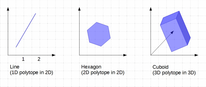
To answer the question what a convex polytope is and for examples, such as a cube, a tetrahedron, a pyramid or the like in 3-dimensional real space, please refer to https://en.wikipedia.org/wiki/Polytope. Also, the polytopes we are interested in shall always be bounded and closed. In some definitions of the term polytope this is already included. I stated this here to make it absolutely clear what we are talking about. For simplicity or as an example one can think of two cubes or boxes for the next sections. Additionally, some samples of polytopes are given in the picture below.
So, let again be \(K\) and \(L \subset \mathbb{R}^{n}\), where \(n \in \mathbb{N}\). The Theorem of Minkowski (https://de.wikipedia.org/wiki/Satz_von_Minkowski) delivers that a bounded, closed convex polytope \(K \subset \mathbb{R}^{n}\) is the convex hull of its extremal points or corners. For example, the convex hull of the eight corners of a 3-dimensional cube is the cube itself.
Please note that I referenced the German Wikipedia site as the Theorem of Minkowski denotes two different theorems in German and English and there is currently no English site for the corresponding theorem on Wikipedia. Apart from that the statement one needs can also be found here https://en.wikipedia.org/wiki/Convex_hull#Convex_hull_of_a_finite_point_set in English.
Now, suppose we have the sets of corners of \(K\) and \(L\). Let us call these sets \(S\) and \(T\), respectively. Also note that the cardinalities of both sets are finite numbers by definition. This leads to the following result for \(K\) and \(S\).
$\begin{align} S & \subseteq K, \\ K & = conv(S) = \{ \sum _{i=1} ^{\vert S \vert} \lambda _{i} s _i \, \vert \, s _i \in S, \lambda _i \geq 0 \, \forall \, i, \sum _{i=1} ^{\vert S \vert} \lambda _i = 1 \} \end{align}$
The same applies for \(L\) and \(T\), respectively.
The main result of this is that we can represent every point of a polytope as a convex combination of its corners and the polytope itself by the convex hull of its corners.
Now, let us add some additional information on convex polytopes we will need in the next section. We define the Minkowski sum and the Minkowski difference of two sets. If we have two sets \(V\) and \(W \subset \mathbb{R}^{n}\) then there Minkowski sum is defined by
$V + W := \{ v + w \, \vert \, v \in V, w \in W \}$
Their Minkowski difference is defined by
$V - W := \{ v - w \, \vert \, v \in V, w \in W \}$
It also applies that the Minkowski sum or difference of two convex sets is again a convex set. Moreover, it applies that the convex hull of the Minkowski sum or difference of two sets is the same as the Minkowski sum or difference of their convex hulls. More information on this can be found here https://en.wikipedia.org/wiki/Minkowski_addition.
This means for our convex polytopes from above that \(K-L\) is a convex set that can be represented by
$K - L = conv(S) - conv(T) = conv(S-T) = $
Also, we want to define \(-W\) for any set \(W \subset \mathbb{R}^{n}\).
$-W := \{ -w \, \vert w \in W \}$
By definition this also means that
$\vert -W \vert = \vert W \vert$
Together with the above we get for any finite set \(V \subset \mathbb{R}^{n}\) the following result.
$\begin{align} -conv(V) & = - \{ \sum _{i=1} ^{\vert V \vert} \lambda _{i} v _i \, \vert \, v _i \in V, \lambda _i \geq 0 \, \forall \, i, \sum _{i=1} ^{\vert V \vert} \lambda _i = 1 \} \\ & = \{ - \sum _{i=1} ^{\vert V \vert} \lambda _{i} v _i \, \vert \, v _i \in V, \lambda _i \geq 0 \, \forall \, i, \sum _{i=1} ^{\vert V \vert} \lambda _i = 1 \} \\ & = \{ \sum _{i=1} ^{\vert V \vert} - \lambda _{i} v _i \, \vert \, v _i \in V, \lambda _i \geq 0 \, \forall \, i, \sum _{i=1} ^{\vert V \vert} \lambda _i = 1 \} \\ & = \{ \sum _{i=1} ^{\vert V \vert} \lambda _{i} (-v) _i \, \vert \, v _i \in V, \lambda _i \geq 0 \, \forall \, i, \sum _{i=1} ^{\vert V \vert} \lambda _i = 1 \} \\ & = \{ \sum _{i=1} ^{\vert V \vert} \lambda _{i} v _i \, \vert \, v _i \in -V, \lambda _i \geq 0 \, \forall \, i, \sum _{i=1} ^{\vert V \vert} \lambda _i = 1 \} \\ & = conv(-V) \end{align}$
Before starting with the next section, the picture below shows a graphical example of the Minkowski sum of two sets in 2-dimensional real space.

Collision Detection
This section will define what collision detection means in this context and how it can be understood. For this reason, we start with some thoughts on the terms collision and colliding.
Suppose one has two arbitrary objects and wants to know if these two objects are colliding or not. Actually, one is interested in the fact if the two objects touch or intersect each other or not. This leads to one possibilty on how one can identify if two objects are colliding or not. What we need to answer the question is the distance between those two objects. In case their distance is 0 the objects are colliding and otherwise, they are not.
Now, assume one has two non-empty sets \(V\) and \(W \subset \mathbb{R}^{n}\). Let \(d\) be a metric on \(\mathbb{R}^{n}\), which means, it applies
$\begin{align} (i) \, & d(v,w) \geq 0, \quad d(v,w) = 0 \Leftrightarrow v = w, \\ (ii) \, & d(v,w) = d(w,v), \\ (iii) \, & d(v,w) \leq d(v,u) + d(u,w), \\ & \forall \, u,v,w \in \mathbb{R}^{n} \end{align}$
This allows us to define the distance \(dist\) between any two points in \(\mathbb{R}^{n}\) using the metric. Furthermore, the distance between the two non-empty sets \(V\) and \(W\) can be defined by
$dist(V,W) := inf \{ d(v,w) \, \vert \, v \in V, w \in W \}$
Also note that in case the sets \(V\) and \(W\) are compact the infimum can be replaced by the minimum.
All in all this is a quite intuitive definition for the distance of two objects and we have a fine method to define explicitly what it means if two objects are colliding or not. Taking the definition of the \(dist\)-function into account, this means that \(V\) and \(W\) are colliding if and only if there is at least a single pair of points \((v,w)\) with \(v \in V\) and \(w \in W\) for which applies \(v = w\). This again can be rewritten as
$v = w \Leftrightarrow v - w = 0, \quad v \in V, w \in W, 0 \in \mathbb{R}^{n}$
This last step is crucial, because it allows to check for the collision of \(V\) and \(W\) using a different criterium. As the above applies \(V\) and \(W\) are colliding if and only if they have at least a single point in common. The last equation means that we can also decide if there is a collision by answering the question:
$Is \, 0 \in (V-W)?$
where \((V-W)\) denotes the Minkowski difference.
Now, taking again the two convex polytopes \(K\) and \(L \subset \mathbb{R}^{n}\) from above, we can state that those objects are colliding if and only if
$\begin{align} & dist(K,L) = 0 \\ \Leftrightarrow \, & 0 \in (K-L) \end{align}$
This leads to another problem for calculating. Due to the definitions of the \(dist\)-function and the Minkowski difference we would have to calculate all distances or differences, respectively, for all pairs of points. Unfortunately, there are uncountably infinite of those.
But this is not the end. Luckily, we can describe the two sets \(K\) and \(L\) using a quite clever system. As we learned before, both sets can be represented by their convex hulls \(conv(S)\) and \(conv(T)\) of their corners \(S\) and \(T\), respectively. Hence, the above can be rewritten as
$\begin{align} & dist(conv(S),conv(T)) = 0 \\ \Leftrightarrow \, & 0 \in (conv(S)-conv(T)) \\ \Leftrightarrow \, & 0 \in (conv(S)+conv(-T)) \end{align}$
This basically means, we are now looking for a representation of \(0 \in \mathbb{R}^{n}\) based on the sum of two convex combinations of the same point, where one convex combination consists of points in \(S\) and the other one of points in \(-T\). This simply leads to a linear system.
$\begin{align} \hat{A}x & = 0, \\ x & \geq 0, \, \sum _{i = 1} ^{\vert S \vert} x _i = 1, \, \sum _{i = \vert S \vert + 1} ^{\vert S \vert + \vert T \vert} x _i = 1 \end{align}$
where \(\hat{A} \in \mathbb{R}^{n \times (\vert S \vert + \vert T \vert)}\) with the elements of \(S\) and \(-T\) being the columns of \(\hat{A}\). Hence, if and only if this linear system has a valid solution, the two polytopes \(K\) and \(L\) are colliding.
What makes this linear system more complicated are the constraints set for \(x\). Fortunately, these have a special form. Looking at the two last constraints one can see that they can be also expressed as products of vectors.
$\begin{align} a _{n+1} x & = 1, \\ a _{n+2} x & = 1, \end{align}$
where the elements \(a _{n+1, i}\) and \(a _{n+2, i}\) of the vectors \(a _{n+1}\) and \(a _{n+2}\) are given by
$\begin{align} a _{n+1, i} & = \left\{\begin{array}{lr} 1 & \forall \, 1 \leq & i & \leq \vert S \vert \\ 0 & \forall \, (\vert S \vert + 1) \leq & i & \leq (\vert S \vert + \vert T \vert) \end{array}\right. \\ a _{n+2, i} & = \left\{\begin{array}{lr} 0 & \forall \, 1 \leq & i & \leq \vert S \vert \\ 1 & \forall \, (\vert S \vert + 1) \leq & i & \leq (\vert S \vert + \vert T \vert) \end{array}\right. \end{align}$
This allows us to rewrite the linear system as
$Ax = b, \quad x \geq 0$
where \(A \in \mathbb{R}^{k \times m}\) is the matrix consisting of \(\hat{A}\) with the additional two equations added at the end given by \(a _{n+1} x = 1\) and \(a _{n+2} x = 1\), \(k = n + 2\), \(m = \vert S \vert + \vert T \vert\), and \(b \in \mathbb{R}^{k}\) is defined by its elements
$b _{i} = \left\{\begin{array}{lr} 0 & \forall \, 1 \leq & i & \leq n \\ 1 & \forall \, (n + 1) \leq & i & \leq k \end{array}\right.$
Again, it applies that this linear system has a valid solution if and only if the two polytopes \(K\) and \(L\) are colliding. Let us call this equation including its constraints the problem \(P1\).
This looks as if we have made things more complicated now. But we will learn that this representation of the collision detection problem is the key. In the next section we will have a look at the simplex method which will lead to the insight that the representation above and the problems the simplex method is able to solve are fitting to each other.
Simplex Method
This section will deal with the issue of how the simplex method can help to solve the previously introduced problem \(P1\) from above. For this at least some knowledge about the simplex method will be needed. An introduction to it can be found here https://en.wikipedia.org/wiki/Simplex_algorithm or here http://mathworld.wolfram.com/SimplexMethod.html.
As the simplex method is a method for linear optimization we start out with a linear optimization problem. Suppose we want to minimize the following function under the given constraints.
$min \, f _{A} (x), \quad f _{A} (x) := e^{T}(b-Ax), \quad Ax \leq b, x \geq 0$
where
$ A \in \mathbb{R}^{k \times m}, \quad e = \left(\begin{array}{lr} 1 \\ 1 \\ \vdots \\ 1 \\ 1 \end{array}\right) \in \mathbb{R}^{k}, \quad b = \left(\begin{array}{lr} 0 \\ \vdots \\ 0 \\ 1 \\ 1 \end{array}\right) \in \mathbb{R}^{k}, \quad k, m \in \mathbb{N}$
being fixed and \(x \geq 0 \in \mathbb{R}^{m}\) is searched for. Let us call this problem \(P2\).
The first thing one might ask for the problem \(P2\) is, if there is any \(x \geq 0 \in \mathbb{R}^{m}\) that fulfills the given constraints. In fact there is one. It is \(x = 0\). This is true because \(b \geq 0\) by definition and it applies that \(0 = Ax \leq b\) for \(x = 0\).
Now, let's have a closer look at the function we want to minimize. We have
$f _{A} (x) := \underbrace{e^{T}}_{> 0}\underbrace{(b-Ax)}_{\geq 0}$
Hence, whatever \(x \geq 0 \in \mathbb{R}^{m}\) fulfills the given constraints and minimizes the given function, for the minimum itself it applies that
$min f _{A} (x) \geq 0 \quad \forall x: Ax \leq b, x \geq 0$
Furthermore, it applies for all \(x \geq 0\) that
$min f _{A} (x) = 0 \Leftrightarrow Ax = b$
Now, take again our collision detection problem \(P1\) from above. For this we do not know if the equation \(Ax = b\) has any solution for \(x \geq 0\) and the polytopes are in fact colliding or not. But, what we have just learnt is quite simple: We do not have to directly solve the equation \(Ax = b\) to decide the collision detection problem, it is enough to solve the optimization problem \(P2\).
Suppose we have found an \(x^{\ast}\) that solves the optimization problem, i.e. it minimizes \(f _{A} (x)\) and fulfills the given constraints. If the resulting minimum is
$f _{A} (x^{\ast}) = 0$
we directly get \(Ax^{\ast} = b\) and hence, the corresponding convex polytopes \(K\) and \(L\) that are represented by the matrix \(A\) and the concerned linear system collide with each other. Otherwise, we get for the minimum that
$f _{A} (x^{\ast}) > 0$
and hence, \(Ax^{\ast} < b\) which due to the optimality of the result includes the information that the polytopes are not colliding.
This is our main result for all the work done so far: The optimization problem can be used to decide the collision detection problem between two convex polytopes: In case the minimum of the given optimization problem is \(0\) the convex poltopes are colliding and otherwise, they are not.
On a side note it should be mentioned that due to the fact that \(b-Ax \geq 0 \in \mathbb{R} ^{k}\) and the given selection of the vector \(e\), it applies that \(f _{A} (x)\) is the 1-norm of the vector \(b-Ax \in \mathbb{R} ^{k}\), i.e.
$f _{A} (x) = e^{T}(b-Ax) = \| (b-Ax) \| _{1}$
Now, what is left to do here is to understand that the simplex method can be used to solve the linear optimization problem \(P2\).
The simplex method is there to solve problems given in a standard form. Unfortunately, there is no standard form defined that is unique. Different authors refer to different standard forms for the simplex method. But, each standard form can be transformed into another one by some defined transformations. For this article, we will refer to the optimization problem given below as the standard form for the simplex method. Minimize
$c^{T}x$
subject to
$Ax = b, \quad x \geq 0$
where \(A \in \mathbb{R}^{k \times m}\), \(b \in \mathbb{R}^{k}\), and \(c \in \mathbb{R}^{m}\) are given by constant values, and \(x \in \mathbb{R}^{m}\) is the vector of variables that is searched for.
This is not quite the form we need to apply the simplex method for problem \(P2\). First we do not have \(c^{T}x\), but instead
$e^{T}(b-Ax) = e^{T}b - e^{T}Ax$
As \(e\) and \(b\) are constants in our problem \(P2\), minimizing the above can be solved by minimizing
$-e^{T}Ax = (-A^{T}e)^{T}x$
Hence, defining
$c:=-A^{T}e$
shows that the function given in problem \(P2\) to be minimized is not an issue. The second issue to solve is the fact that in problem \(P2\) we have the constraints
$Ax \leq b$
instead of
$Ax = b$
Fortunately, the simplex method can be also applied to problems with the given inequality constraints. This is done by introducing so called slack variables. For each line one slack variable is introduced. In case of our problem \(P2\) we introduce \(k\) slack variables to change the inequalities to equalities. Having those slack variables in mind and adopting the linear system for those, we can rewrite the inequality constraints in the linear system as
$\tilde{A}\tilde{x} = b$
where \(\tilde{A} \in \mathbb{R}^{k \times q}\), \(\tilde{x} \in \mathbb{R}^{q}\) with \(q = m + k\), \(I _k \in \mathbb{R}^{k \times k}\) being the identity matrix, and
$\tilde{A} := \left( A, I _k \right), \quad \tilde{x} := \left( \begin{array}{lr} x \\ 0 \\ \vdots \\ 0 \\ 1 \\ 1 \end{array} \right), \, x \in \mathbb{R}^{m} $
Moreover, for this last linear system we also already know a valid solution that is given by applying \(x = 0 \in \mathbb{R}^{m}\) in the above. Hence, this linear system can be transferred to a simplex tableau and we can directly apply the simplex method to calculate a solution.
For more details on this, refer for example to http://en.wikipedia.org/wiki/Simplex_algorithm and further references found there.
Now, we have everything we need to answer our question if two given convex polytopes \(K\) and \(L \subset \mathbb{R}^{n}\) are colliding or not. In the next section, we will therefore list the algorithm to be implemented.
Algorithm
After all the theory above, we get to the algorithm itself. It turns out that - given an implementation for the simplex method - the algorithm is quite easy.
Algorithm to decide if two convex polytopes \(K\) and \(L \subset \mathbb{R}^{n}\) are colliding:
- Get the corners of both polytopes.
- Check if any polytope or its set of corners is the empty set.
- If the above is true, there is no collision as there is nothing to collide with - goto END.
- Check if both polytopes or their sets of corners, respectively, consist only of one single point.
- If so, check both single points for equality.
- If both points are the same, the polytopes collide - goto END.
- If both points are not the same, the polytopes do not collide - goto END.
- If at least one polytope has two ore more corners, apply the simplex method to decide for the collision as described above.
- If the resulting minimum is 0, the two polytopes are colliding - goto END.
- If the resulting minimum is greater than 0, the two polytopes are not colliding - goto END.
- END.
Code
The code introduced here is just a basic implementation of the algorithm and is done for 3-dimensional real space. I suppose there might and will be other and better implementations of the simplex method out there. One just needs to adapt and use them. Nevertheless, the given code is working and can be downloaded together with an application for testing.
The code itself consists of actually three classes, only one is really interesting of. Two classes are actually there to wrap the collision detection algorithm implemented and to facilitate usage. Those two classes are the classes ConvexPolyhedron.cs and ConvexPolyhedronExtensions.cs. The algorithm itself is fully implemented in the class LinearProgramming.cs.
ConvexPolyhedron.cs
#region Usings (3)
using System.Collections.Generic;
using System.Windows.Media.Media3D;
using System.Xml.Serialization;
#endregion // Usings (3)
namespace CollisionDetection
{
public class ConvexPolyhedron
{
#region Public Non-Static Properties (2)
[XmlElement]
public string Name { get; set; } = string.Empty;
[XmlArray]
public HashSet<Point3D> Corners { get; set; } = new HashSet<Point3D>();
#endregion // Public Non-Static Properties (2)
}
}
ConvexPolyhedronExtensions.cs
#region Usings (4)
using System;
using System.Collections.Generic;
using System.Linq;
using System.Windows.Media.Media3D;
#endregion // Usings (4)
namespace CollisionDetection
{
public static class ConvexPolyhedronExtensions
{
#region Public Static Extension Methods (2)
public static bool CollidesWith(this ConvexPolyhedron convPolyA,
ConvexPolyhedron convPolyB)
{
return LinearProgramming.AreColliding(convPolyA?.Corners, convPolyB?.Corners);
}
public static bool IsSubsetOf(
this ConvexPolyhedron setToTest,
ConvexPolyhedron supposedSuperset)
{
bool result;
if ((null == setToTest) || (null == setToTest.Corners))
{
throw new ArgumentNullException("setToTest",
"The object that represents the set that is tested"
+ " for being a subset is null.");
}
if ((null == supposedSuperset) || (null == supposedSuperset.Corners ))
{
throw new ArgumentNullException("supposedSuperset",
"The object that represents the superset for testing is null.");
}
if (setToTest.Corners.Any())
{
if (supposedSuperset.Corners.Any())
{
int loop;
loop = 0;
result = true;
while (result && (setToTest.Corners.Count > loop))
{
result &= LinearProgramming.AreColliding(
new HashSet<Point3D>()
{
setToTest.Corners.ElementAt(loop)
},
supposedSuperset.Corners);
loop++;
}
}
else
{
result = false;
}
}
else
{
result = !supposedSuperset.Corners.Any();
}
return result;
}
#endregion // Public Static Extension Methods (2)
}
}
LinearProgramming.cs
#region Usings (4)
using System;
using System.Collections.Generic;
using System.Linq;
using System.Windows.Media.Media3D;
#endregion // Usings (4)
namespace CollisionDetection
{
public static class LinearProgramming
{
#region Private Constants (3)
private const int DIMENSION = 3;
private const int NUMBER_OF_CONVEXITY_CONSTRAINTS = 2;
private const int NUMBER_OF_EQUATIONS = LinearProgramming.DIMENSION
+ LinearProgramming.NUMBER_OF_CONVEXITY_CONSTRAINTS;
private const int NUMBER_OF_SLACK_VARIABLES = LinearProgramming.DIMENSION
+ LinearProgramming.NUMBER_OF_CONVEXITY_CONSTRAINTS;
#endregion // Private Constants (3)
#region Public Static Read-Only Properties (1)
public static readonly double DEFAULT_EPSILON = 0.0001;
#endregion // Public Static Read-Only Properties (1)
#region Private Static Members (1)
private static double _epsilon;
#endregion // Private Static Members (1)
#region Public Static Properties (1)
public static double Epsilon
{
get { return _epsilon; }
set
{
if (0 >= value)
{
throw new ArgumentException("The applied accuracy must not be 0 or less.");
}
_epsilon = value;
}
}
#endregion // Public Static Properties (1)
#region Static Constructor (1)
static LinearProgramming()
{
Epsilon = LinearProgramming.DEFAULT_EPSILON;
}
#endregion //Static Constructor (1)
#region Public Static Methods (4)
public static bool AreColliding(ISet<Point3D> convPolyA, ISet<Point3D> convPolyB)
{
bool result;
if (null == convPolyA)
{
throw new ArgumentNullException("convPolyA",
"The given set of points representing the first convex polyhedron is null.");
}
if (null == convPolyB)
{
throw new ArgumentNullException("convPolyB",
"The given set of points representing the second convex polyhedron is null.");
}
if (!convPolyA.Any() || !convPolyB.Any())
{
result = false;
}
else
{
if ((1 == convPolyA.Count) && (1 == convPolyB.Count))
{
Point3D pointA = convPolyA.ElementAt(0);
Point3D pointB = convPolyB.ElementAt(0);
result = ((pointA.X - pointB.X) < LinearProgramming.Epsilon)
&& ((pointA.Y - pointB.Y) < LinearProgramming.Epsilon)
&& ((pointA.Z - pointB.Z) < LinearProgramming.Epsilon);
}
else
{
result =
LinearProgramming.PerformSimplexMethod(
LinearProgramming.CreateInitialTableau(
convPolyA, convPolyB)) < LinearProgramming.Epsilon;
}
}
return result;
}
public static double[,] CreateInitialTableau(
ISet<Point3D> convPolyA, ISet<Point3D> convPolyB)
{
double[,] tableau = new double
[LinearProgramming.NUMBER_OF_EQUATIONS + 1,
convPolyA.Count + convPolyB.Count
+ LinearProgramming.NUMBER_OF_SLACK_VARIABLES + 1];
for (int k = 0; k < convPolyA.Count; k++)
{
tableau[1, k] = convPolyA.ElementAt(k).X;
tableau[2, k] = convPolyA.ElementAt(k).Y;
tableau[3, k] = convPolyA.ElementAt(k).Z;
tableau[4, k] = 1.0;
tableau[5, k] = 0.0;
}
for (int k = 0; k < convPolyB.Count; k++)
{
int k_shifted = k + convPolyA.Count;
tableau[1, k_shifted] = -convPolyB.ElementAt(k).X;
tableau[2, k_shifted] = -convPolyB.ElementAt(k).Y;
tableau[3, k_shifted] = -convPolyB.ElementAt(k).Z;
tableau[4, k_shifted] = 0.0;
tableau[5, k_shifted] = 1.0;
}
for (int k = 0; k < (convPolyA.Count + convPolyB.Count); k++)
{
tableau[0, k] = 0.0;
for (int i = 1; i < tableau.GetLength(0) ; i++)
{
tableau[0, k] -= tableau[i, k];
}
}
for (int k = (convPolyA.Count + convPolyB.Count);
k < (convPolyA.Count + convPolyB.Count
+ LinearProgramming.NUMBER_OF_SLACK_VARIABLES);
k++)
{
tableau[0, k] = 0.0;
for (int i = 1; i < tableau.GetLength(0); i++)
{
tableau[i, k] =
((k - convPolyA.Count - convPolyB.Count + 1) == i)
? 1.0 : 0.0;
}
}
tableau[0, convPolyA.Count + convPolyB.Count
+ LinearProgramming.NUMBER_OF_SLACK_VARIABLES] = 0.0;
for (int i = 1; i < tableau.GetLength(0); i++)
{
tableau[i, convPolyA.Count + convPolyB.Count
+ LinearProgramming.NUMBER_OF_SLACK_VARIABLES]
= (LinearProgramming.DIMENSION >= i) ? 0.0 : 1.0;
tableau[0, convPolyA.Count + convPolyB.Count
+ LinearProgramming.NUMBER_OF_SLACK_VARIABLES]
-= tableau[i, convPolyA.Count + convPolyB.Count
+ LinearProgramming.NUMBER_OF_SLACK_VARIABLES];
}
return tableau;
}
public static double PerformSimplexMethod(double[,] tableau)
{
double infimum;
int loop;
int pivotColumn;
int pivotRow;
int numberOfColumns = tableau.GetLength(1);
int numberOfRows = tableau.GetLength(0);
int limitOfLoops = numberOfColumns * numberOfRows;
int baseSlackVariableIndex = tableau.GetLength(1)
- LinearProgramming.NUMBER_OF_EQUATIONS - 1;
int[] basicIndices = new int[LinearProgramming.NUMBER_OF_EQUATIONS];
infimum = 2.0;
for (loop = 0; loop < LinearProgramming.NUMBER_OF_EQUATIONS; loop++)
{
basicIndices[loop] = baseSlackVariableIndex + loop;
}
SelectPivotByBlandsRule(tableau, basicIndices, out pivotRow, out pivotColumn);
while ((infimum >= LinearProgramming.Epsilon)
&& (pivotColumn < numberOfColumns)
&& (pivotRow < numberOfRows)
&& (limitOfLoops > loop))
{
if ((0 > pivotColumn) || (0 > pivotRow))
{
throw new ArgumentException("Something went wrong!"
+" The pivot selection failed with an error!!!");
}
basicIndices[pivotRow - 1] = pivotColumn;
double pivot = tableau[pivotRow, pivotColumn];
for (int i = 0; i < numberOfColumns; i++)
{
tableau[pivotRow, i] = i == pivotColumn ? 1.0 : tableau[pivotRow, i] / pivot;
}
for (int k = 0; k < numberOfRows; k++)
{
if (k != pivotRow)
{
double temp = tableau[k, pivotColumn];
for (int i = 0; i < numberOfColumns; i++)
{
tableau[k, i] = i == pivotColumn
? 0.0
: tableau[k, i] - temp * tableau[pivotRow, i];
}
}
}
infimum = -tableau[0, numberOfColumns - 1];
SelectPivotByBlandsRule(tableau, basicIndices, out pivotRow, out pivotColumn);
loop++;
}
return infimum;
}
public static void SelectPivotByBlandsRule(
double[,] tableau,
int[] basicIndices,
out int row,
out int column)
{
int loop;
int numberOfPivotRows;
int numberOfPivotColumns;
int lastColumn;
int smallestBasicIndex;
double quotient;
IList<int> possibleRows = new List<int>();
row = -1;
column = -1;
loop = 0;
numberOfPivotColumns = tableau.GetLength(1) - 1;
while ((tableau[0, loop] + LinearProgramming.Epsilon >= 0)
&& (numberOfPivotColumns > loop))
{
loop++;
}
column = loop;
if (numberOfPivotColumns <= column)
{
row = tableau.GetLength(0);
column = tableau.GetLength(1);
}
else
{
loop = 1;
numberOfPivotRows = tableau.GetLength(0);
lastColumn = tableau.GetLength(1) - 1;
quotient = double.MaxValue;
while (numberOfPivotRows > loop)
{
if (0 < tableau[loop, column])
{
if ((tableau[loop, lastColumn] / tableau[loop, column]) < quotient)
{
quotient = (tableau[loop, lastColumn] / tableau[loop, column]);
possibleRows.Clear();
possibleRows.Add(loop);
}
else if (Math.Abs(tableau[loop, lastColumn] / tableau[loop, column]
- quotient) < LinearProgramming.Epsilon)
{
possibleRows.Add(loop);
}
}
loop++;
}
if (possibleRows.Any())
{
if (1 == possibleRows.Count)
{
row = possibleRows[0];
}
else
{
loop = 1;
smallestBasicIndex = tableau.GetLength(1);
while (possibleRows.Count > loop)
{
if (smallestBasicIndex > basicIndices[possibleRows[loop]-1])
{
row = possibleRows[loop];
smallestBasicIndex = basicIndices[possibleRows[loop]-1];
}
loop++;
}
}
}
if (0 > row)
{
row = tableau.GetLength(0);
column = tableau.GetLength(1);
}
}
}
#endregion // Public Static Methods (4)
}
}
Performance
Regarding performance, I personally have no numbers comparing this algorithm to another one solving the collision detection problem for convex polytopes. So, the only thing I can state here is some general results that base on the simplex method and can therefore be also found in related literature or for example here http://mathworld.wolfram.com/SimplexMethod.html.
The simplex method itself is in general a method with an exponential performance, i.e.
$O(exp(k))$
where \(k \in \mathbb{N}\) denotes the number of equations of the linear system that defines the constraints for the optimization problem. Fortunately, in practice it shows and can also be proved for some defined situations that the simplex method has a linear performance. Hence, if no quite special situation is constructed, one can state that the collision detection algorithm introduced will solve the issue in
$O(k)$
Nevertheless, this means that one should limit the number of iterations performed by an implementation of the simplex method to not ruin the performance if one runs into trouble.
Remarks
As a last part of this article regarding its pure content there are a few things that shall be mentioned because they must be taken into account upon deciding to use this algorithm or not.
First of all, there is the question for the performance. As already stated, in practical applications the performance should be linear and hence, quite fine. Nevertheless, an exponential behaviour cannot be excluded. Additionally, there are faster, but more coarse tests for collision detection especially if the concerned polytopes are quite far from each other. Therefore, if used in a collision detection system, one should start with e.g. a collision detection test based on bounding boxes or bounding spheres of the polytopes. If those tests imply a collision, one should use an improved, more accurate test, such as the one described here.
One advantage of the given algorithm performing a theoretically exact collision detection test for convex polytopes is that one does not need a specific form of the polytope or orientation information. The corners of the polytopes contain all information needed by this algorithm.
As already suggested the algorithm is only theoretically exact. What is meant by this is quite easy. Due to the inaccuracy of computers when performing calculations using floating point numbers a meaningful stop criteria for the simplex method based on the accuracy is needed, i.e. it must be made a concrete decision on the accuracy that is the limit for distinguishing two floating point numbers. For example, an accuracy of 0.001 might be enough and hence, a collision is assumed, if the simplex method returns a result with a minimum value below 0.001 instead of being exactly 0.
Another issue that can arise due to numerical inaccuracy is the one of infinite cycling without progress. Bad implementations of the simplex method can lead to cycles in the tableaux calculated. These cycles can theoretically be prevented by using dedicated selection algorithms upon selecting the pivot element for the next step in the simplex method. For example, in the implementation coded here Bland's rule (https://en.wikipedia.org/wiki/Bland's_rule) is used, which can be proved for that it does not lead to cycles. Unfortunately, erasment of numbers in the tableaux due to numerical inaccuracy can also lead to cycles even if an algorithm for selecting pivot elements is used that can be proved to lead to a cycling-free calculation.
What must also be emphasised here is that the algorithm introduced can decide if there is a collision between two polytopes or not. What it does not do is calculating the distance between the two polytopes. The function to be minimized of the problem \(P2\) from above only delivers - as already mentioned - the 1-norm of the vector \(b-Ax \in \mathbb{R}^{k}\). Fortunately, this at least allows us to get a more or less accurate estimation for the distance of the two polytopes. In case the two polytopes are colliding, the distance is clearly \(0\) as shown above. In case the two polytopes are not colliding, the calculated minimum \(>0\) gives us the information that for all other vectors \(\tilde{y} := b - A\tilde{x}\in \mathbb{R}^{k}\) fulfilling the constraints of problem \(P2\) it applies
$\| \tilde{y} \| _1 \geq min f _{A} (x)$
This is especially true for such vectors \(\tilde{y} \in \mathbb{R}^{k}\) of type
$\tilde{y} = \left(\begin{array}{lf} y \\ 0 \\ 0 \end{array}\right) \quad y \in \mathbb{R}^{n}$
for which it applies that \(y \in (K-L)\) due to the fact that the last two elements of the vector \(\tilde{y}\) are \(0\) and hence, fulfilling the equations for being an element of the Minkowski difference of the two convex polytopes. Therefore, if the calculated minimum is \(>0\) it applies for all such \(y \in (K-L)\) that their 1-norm is greater or equal to the minimum.
As stated, this estimation is more or less accurate, depending on the concrete polytopes given. Moreover, one will never get a minimum value \(>2\), due to the fact that one starts the calculation with the simplex method with \(x=0\), performs only steps that do not worsen the result, and it is
$\| b-Ax \| _1 = \| b-0 \| _1 = \| b \| _1 = 2$
Another issue is that the estimation is based on the 1-norm. Normally, the distance in real space is measured using the Euclidean-norm or 2-norm, because it fits intuitively to our perception of the real world. As we only work with finite-dimensional real spaces we can now use the equivalence of the norms to get an estimation for the distance measured in the 2-norm (for more details on this, refer to e.g. https://en.wikipedia.org/wiki/Lp_space#The_p-norm_in_finite_dimensions). For any \(z \in \mathbb{R}^{k}\) it applies that
$ \sqrt{k} \| z \| _2 \geq \| z \| _1 \geq \| z \| _2$
which leads to the following result for estimating the distance between \(K\) and \(L\) in the 2-norm - based on the prerequisite that the defining metric for the \(dist\)-function is the one induced by the 1-norm - by rewriting the inequalities in case the two polytopes are not colliding and by using a solution of the optimization problem called \(x^{\ast}\):
$ dist(K,L) \geq \| (b-Ax^{\ast}) \| _1 \geq \| (b-Ax^{\ast}) \| _2 \geq \frac{1}{\sqrt{n}} \| (b-Ax^{\ast}) \| _1 > 0$
Hence, one can directly estimate the distance in the 2-norm by only using the calculated minimum (refer to the next to last inequality above) and use this as estimation for the distance of the polytopes. Also, note the adaptation of \(k\) by replacing it with the value \(n=k-2\) in the inequality. This can be done because for all possible points in \(K-L\) the last two elements of the resulting minimum vector must be \(0\) and the minimum value of the 2-norm of such a vector in case of a defined and given 1-norm value is given by a uniform distribution of the value on the first \(n=k-2\) elements, i.e. by the vector
$z = \left(\begin{array}{lf} z _1 \\ \vdots \\ z _n \\ 0 \\ 0 \end{array}\right) \quad z _i := \frac{1}{n} \| (b-Ax^{\ast}) \| _1 , \, \, \forall i=1, \cdots, n$
Unfortunately, this value is dependent on the dimension \(n\) of the related real space. Changing the implementation of the simplex method to not only return the calculated minimum, but also the determined \(x^{\ast}\) itself will not help (as previously stated here, which was wrong). This is the case because \(x^{\ast}\) need not to be unique and therefore, the resulting minimum vector and its 2-norm is not ensured to be the one with the smallest value of (possibly) existing solutions.
Regarding the implementation coded here it shall be mentioned that it uses the standard simplex method, but there exists a revised simplex method which is equivalent to the standard simplex method and more efficient in sense of computing. Refer to e.g. https://en.wikipedia.org/wiki/Revised_simplex_method for more information.
Apart from everything stated so far I want to add a remark on the Gilbert–Johnson–Keerthi distance algorithm (refer to e.g. https://en.wikipedia.org/wiki/Gilbert-Johnson-Keerthi_distance_algorithm) as this might be important. Thanks to Kenneth Haugland who mentioned it in the comments.
If you have a look at the Gilbert–Johnson–Keerthi distance algorithm you will see that it is better in the sense that it delivers not only the collision result, but in case there is no collision it also delivers the distance in the 2-norm which is normally better than the above. Apart from that, the Gilbert–Johnson–Keerthi distance algorithm also has a linear performance that can almost be put down to constant under certain circumstances given a proper implementation. It is also a different algorithm that the one presented here, but it is true that both are using the same concepts regarding set calculation, namely the Minkowski difference. My personal opinion is that as the Gilbert–Johnson–Keerthi distance algorithm additionally needs some so called supporting functions for its calculations the algorithm presented here is easier to understand and implement at the very beginning as it only relies on the corners of the polytopes. Therefore, I hope it could be a good starting point for people who are interested in collision detection.
A final remark shall be given on using the simplex method for collision detection. This is also not a brand new idea. Referring to Real-Time Collision Detection by Christer Ericson, chapter 9 (note that I referenced the webpage, the book can be found and bought easily) one can see that the idea is already there for a while. But, different to that one, the algorithm used here is not based on halfspaces but on the corners of the polytopes, leading to a totally different set of equations to be solved using the simplex method.
References
The references listed here are grouped and ordered by appearance in the article. I want to thank Prof. Dr. Andreas Kirsch of the KIT - Karlsruher Institute of Technology (former University of Karlsruhe (TH), Germany) because the code of the algorithm presented here is based on lecture notes from his lecture Optimierungstheorie held in the summer semester 2005 in Karlsruhe. I also want to thank John Jiyang Hou for his article that actually pushed me to take the time and write this one and Kenneth Haugland for his comment below that convinced me to at least add a remark on the Gilbert–Johnson–Keerthi distance algorithm and the book about real-time collision detection by Christer Ericson.
Code Project
Wikipedia
Mathworld Wolfram
Christer Ericson
KIT - Karlsruher Institute of Technology (former University of Karlsruhe (TH), Germany)
History
Please find the history of the article below. The order is from latest to oldest.
June 7th, 2016: Important change regarding distance estimation and Gilbert–Johnson–Keerthi distance algorithm
- Reworked remarks section to remove a wrong statement about distance estimation in the 2-norm
- Added information in remarks section to improve the distance estimation in the 1-norm
- Added information in the remarks section about the Gilbert–Johnson–Keerthi distance algorithm
- Updated references section to latest changes
June 5th, 2016: Minor changes
- Fixed failure in equation in remarks section that missed an operation.
June 2nd, 2016: Minor changes
- Fixed typos and spelling mistakes found
May 21st, 2016: Minor changes
- Adjusted initialization of instances of type ConvexPolyhedron
- Updated code files and program after made changes in code
- Tried to fix the set tags
May 20th, 2016: Made some minor fixes
- Fixed typos found
- Adjusted misleading comment of Corners property in ConvexPolyhedron.cs
- Clarified distance estimation in remarks section by using a minimal solution called (x^{\ast}\)
- Removed VS2013 tag as C#6.0 is used in code
- Code files are not adjusted and program was not re-compiled regarding the change of the comment simply because I am currently troubleshooting my development PC
May 20th, 2016: Initial version date
- Release date of the initial version
My name is Andreas Michael Kreuzer and I was born in a small town in Baden-Württemberg, Germany. My 'coding career' started around 1989 on a CPC 6128. I got involved with coding the first time by actually copying code from books or magazines to the CPC to get computer games running. Also, I started to love mathematics about the same time.
After finishing school and doing my military service I started to study computer science as a major at the University of Karlsruhe, Germany. Later on I added also mathematics as a major and finally graduated in both computer science and mathematics. Then - while already working - I participated in an additional program at the German Graduate School of Management and Law in Heilbronn, Germany and got an additional master in business law. Basically, I was fascinated in the fact how much the work of a mathematician and a jurist coincide.
I started to work as a software developer after graduating in Karlsruhe and I am doing this for almost eight years now. After being engaged with different companies I got self-employed and work as a freelancer since beginning of 2016. My main focus is on the C/C++ and C# development.
In my spare time I enjoy jogging, juggling, hiking, and especially spending time with my wife, my little son, and my friends.


 General
  News
News  Suggestion
  Question
  Bug
Bug  Answer
  Joke
Joke  Praise
  Rant
Rant  Admin
Admin 


